Artículo de investigación científica y tecnológica

Evaluation of nonlinear Iterative methods on pipe network

Evaluación de métodos iterativos no lineales en redes de tuberías

0000-0002-0624-5813Guilherme da Silva Teixeira^I  , 0000-0002-9587-8697Guillermo Vilalta-Alonso^{II  *}  , 0000-0002-1239-1040Lourival J. Mendes N^III 

^IUniversidade Federal de São João del-Rei. Energy Engineering Master Program. São João del-Rei, Minas Gerais, Brazil

^IIUniversidade Federal de São João del-Rei. Thermal Sciences and Fluids Department. São João del-Rei, Minas Gerais, Brazil

^IIIUniversidade Federal de Itajubá. Grupo de Estudos em Tecnologias de Conversão de Energia-GETEC. Itajubá, Minas Gerais/Brazil

Abstract

The analysis and design of pipe networks is usually a very complex task and depending of many factors. The paper here presented explores issues related to the accuracy and robustness of three iterative nonlinear methods used for designing pipe networks: Hardy Cross method, Gradient method and Newton-Raphson method. The last two methods are implemented in EPANET and Matlab, through the fsolve function. In order to evaluate the performance of each numerical method, three pipe networks, were assessed. No differences in the results were found by using fsolve (of MatLab) and Hardy-Cross methods. However, the EPANET results show differences up to 115% regarding other two methods. This behavior can be explained by the magnitude of head loss and the flow rate in some tubes of the network with errors close to the errors set up and by the Nodal Newton-Raphson method used at EPANET’s code. The Hardy Cross method proved to be robust on three evaluated cases

Key words: nonlinear methods, pipe network; EPANET; Hardy Cross method; Newton-Raphson technique

Resumen

El proyecto y análisis de redes de tuberías suele ser una tarea muy compleja que depende de muchos factores. El trabajo aquí presentado explora cuestiones relacionadas con la precisión y la robustez de tres métodos iterativos no lineales utilizados para proyectar redes de tuberías: el método Hardy Cross, el método de Gradiente y el método Newton-Raphson. Los dos últimos métodos se implementan en EPANET y Matlab, a través de la función fsolve. Para evaluar el desempeño de cada método numérico, se evaluaron tres redes de tuberías. No se encontraron diferencias en los resultados cuando la función fsolve (de MatLab) y el método Hardy-Cross son utilizados. Sin embargo, los resultados de EPANET muestran diferencias de hasta un 115 % con respecto a los otros dos métodos. Este comportamiento puede explicarse debido a la magnitud de la pérdida de carga y del caudal en algunos tubos de la red, con errores próximos al error establecido para la convergencia y, también, por el método Nodal Newton-Raphson utilizado en el código de EPANET. El método de Hardy Cross demostró ser robusto en tres casos evaluados.

Palabras-clave: métodos no lineales; redes de tuberías; EPANET; método Hardy Cross; técnica de Newton-Raphson

Introduction

Water distribution networks are designed and calculated for many purposes in addition to its main application: water supplying for human consumption at adequate pressure and flow rate. Piped water is also used in many others applications as washing, sanitation, irrigation and firefighting. The networks design should meet some important criteria related to maximum demands ^[1]. It is noticed that the calculation of the water networks must be done properly, being this the reason why some methods have been proposed in the literature.

Hardy Cross was the pioneer by proposing two methods for approaching the networking solution. Firstly, the flows in the pipes in a network always satisfy the condition that the total flow into and out of each junction is zero, and these flows are successively corrected to satisfy the condition of zero total change of head around each circuit. Secondly, the total change of head around each circuit is always equals zero, and the flows in the pipes of the circuit are successively adjusted so that the total flow into and out of each junction finally approaches or becomes zero ^[2].

An example of the successful application of the Hardy Cross Method was reported in ^[3] where it was carried about an analysis of the water distribution at the community of Macundú in Rio de Janeiro State, Brazil. The method was consistent and allowed the determination of fundamental parameters of the network, flow, and pressure, to achieve the physical distribution of the water system for the community.

Although the Hard Cross method is widely accepted and used, it has some limitations. Convergence problems are the main limitation that occurs due to a bad guess leading to a very slow convergence or divergence ^[4]. According to ^[5], an approach to get over this limitation is the solution of a network, via linear theory, in which the continuity equations at nodes and energy conservation for each loop are solved simultaneously and the discharge in each pipe is directly obtained. There is no need to guess initial discharges to satisfy the continuity equations at nodes. Subsequent developments of this algorithm, which led to commercial software KYPIPE was due to the implementation of the Newton-Raphson method ^[6].

Later, the Hardy Cross method was modified ^[7] and the results were compared with their previous work ^[8], when the authors modified the Newton-Raphson technique and compared it also with other works of the literature and with EPANET ^[7]. In conclusion, for complex networks, the modified Hardy Cross method was more efficient than the traditional Newton-Raphson method and it takes less time between iterations than the original Hardy Cross method. The results obtained matched well with the ones from EPANET.

The Newton-Raphson method can be also applied using a Trust Region Dogleg technique to supply some convergence issues and turn it fast. It is applied using the function fsolve from Matlab which is specially designed to solve nonlinear equations ^[9].

A new method to determine flows in pipe networks with rings was developed in ^[10]. This new method is constituted by formulating a nonlinear system of algebraic equations that is solved through fsolve function. The results obtained were very similar to those that can be found on literature, as well as the mass balance was satisfied and the sum of the pressure drop in the pipes in any closed circuit was zero.

The fsolve can fail to convergence when trying to solve an equation, for example, that the user attempts to get high accuracy by setting tolerances to very small values. The fsolve function might fail to converge for equations with discontinuous gradients, such as absolute value ^[9].

The global gradient method ^[11] is a highly popular method, implemented in EPANET software. In this method, energy equations are combined with the nodal equations and are simultaneously solved to estimate the nodal heads and flow discharge. Here, like the methods of “simultaneous loop” and "linear theory", nonlinear energy equations are linearized by using Taylor series expansion. However, they are solved using an optimal and reversal scheme, which applies the inverse of the coefficients matrix ^[6].

Recently, ^[12] compared EPANET with the modified Hunter model in an analysis of the water distribution network in buildings. At the end of his experiments, the authors showed that EPANET is very effective, noting a percentage difference in the results from 0.24% to 1.06% between the software and the Hunter method.

Some published researches that show some EPANET issues leading to mistaken results ^[13, ^14]. In ^[13], the authors proposed a method for automatic functional testing in hydraulic simulators. The method is based on using genetic algorithms to search for network parameter values in which the simulator under test computes solutions that do not satisfy the governing network equations.

The testing program was first applied to a network, with 351 variable parameters, by using the EPANET package. The incorrect solutions detected involved pipes with a head loss in order of 10−4 m and less; for such pipes, the EPANET computed total heads at the pipe ends, the predominant case being a nonzero pipe flow at equal total heads. These solutions are, in part, due to loss of significant digits since the computed data are transferred from the EPANET simulator. They may also occur because in an EPANET solution, the flow through a tube and the heads at its ends are not directly related by the head loss-flow relationship. Because of small flows and/or low pipe resistances, a linear head loss-flow relationship has been used in the EPANET solver instead of Hazen-Williams to avoid singular matrices.

Agreeing with ^[13, ^14] stated that the EPANET software uses a demand-driven approach to simulate water distribution systems. The EPANET solver uses the Cholesky decomposition to compute the solution of a system of linear equations. However, under deficient pressure conditions the EPANET results are inaccurate. Therefore, in these scenarios a pressure-driven model is required. Embedding a pressure-driven model in the EPANET solver allows the computation of the available demand as a function of the current pressure and allows account for leakage at pipe level. Nevertheless, these increasing modelling capabilities have a side effect: new terms for the system coefficients matrix and the possibility of the matrix being positive indefinite. This requires a new approach to reach convergence: a numerical factorization applicable to indefinite matrices and relaxation coefficients to improve convergence ^[14].

The Hardy Cross method and EPANET were used to create a simple analysis procedure and design of a pipe network ^[15]. The authors concluded that Hardy Cross's method places more emphasis on the effectiveness of the pipe network design, being a simpler method, however it requires more interactions than EPANET.

Taking into account previous discussion regarding advantages and limitations of the different methods used to compute the main variables related to the design of pipes networks, in this paper a comparative analysis about the accuracy and robustness of different methods in calculating three pipe networks is carried out. The three methods are Hardy Cross method, EPANET software and the tool fsolve from Matlab.

Materials and Methods

Problem description

Some methods used to solve pipe networks have issues on their results accuracy because of the amount of unknowns mainly when the number of unknowns is high, in other words, when the network has many tubes, junctions, demands, rings, etc. ^[16, ², ^3]. Other sort of incorrect solution occurs when the head loss is 10-4 m or less and when the flow and/or the resistance are low. In these cases, the EPANET, for example, changes the head loss-flow relationship (Hazen-Williams, Darcy-Weisbach) for a linear one ^[13]. When the stop criterion is too small, consequently, the method could not converge; or if the stop criteria is too high, it generates a wrong result ^[6, ^13].

Because of these limitations, the numerical methods analyzed in this work were assessed considering three different cases in order of complexity, which means, an increase number of pipes, the addition of pumps as well as demands and reservoirs, in order to compare the results accuracy among Hardy-Cross Method, EPANET and Matlab’s tool, fsolve.

Case 01

It consists in 5 tubes, 1 demand and 2 reservoirs, which leads to 2 rings as shown in figure 1.

Fig. 1 First Case pipe network. Source: modified version of ^[16]  

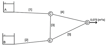
Water flows through the new galvanized iron tubes network. The material and roughness values used on the simulation were taken as the recommended for commercial tubes ^[17]. The reservoir "A" is at an elevation of 15 m and reservoir "B" to a high of 2 m, according to the reference at node “D”. The demand of the system is 0,075 m³/s. All the relevant data for modeling the case are described on table 1 and table 2.

Table 1 Data Case 1. Source: modified version of ^[16]  

Tube	L [m]	D [m]	e [m]	/
1	500	0,3	1,5x10^-4	0
2	600	0,25	1,5x10^-4	0
3	50	0,15	1,5x10^-4	10
4	200	0,25	1,5x10^-4	2
5	200	0,30	1,5x10^-4	2

Table 2 Data for node identify, node elevation and demands, Case 01. Source: modified version of ^[16]  

Node	Elevation [m]	Demand [m³/s]
A	15	0
B	2	0
C	4	0
D	0	0,075
E	1	0

Case 02

It consists in 14 pipes, 5 demands, 3 reservoirs, 4 valves and 1 pump, which forms 5 rings as can be seen in figure 2.

Source: Modified version from ^[18]

Fig. 2 Second Case pipe network. 

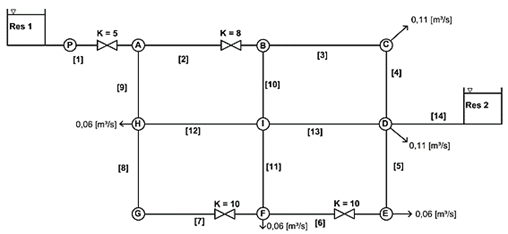
The pump can be described by the equation 1 where HP as Pump’s Head [m], and QP and Pump’s Flow [m³/s]. The water flows through a pipe network of new commercial steel tube, and the roughness is in accordance to the recommended ones ^[17]. Data about pipe identifiers, pipe lengths, pipe diameters, absolute roughness, the singular head loss, nodes identifiers, nodes highs and demands are shown on tables 3 and 4.

[TeX:] H _p = -3.405 x 10 ^-7 Q ² + 166 (1)

Where Q is the demand [m3/h] and H is the head [m]

Table 3 Data for Case 02. Source: Modified version from ^[18]  

Tube	L [m]	D [m]	e [m]
1	1500	0,4	4,6x10 ^-5	5
2	610	0,35	4,6x10 ^-5	8
3	914	0,35	4,6x10 ^-5	0
4	760	0,35	4,6x10 ^-5	0
5	610	0,35	4,6x10 ^-5	0
6	610	0,35	4,6x10 ^-5	10
7	61	0,15	4,6x10 ^-5	10
8	975	0,30	4,6x10 ^-5	0
9	760	0,35	4,6x10 ^-5	0
10	610	0,35	4,6x10 ^-5	0
11	457	0,30	4,6x10 ^-5	0
12	914	0,35	4,6x10 ^-5	0
13	610	0,35	4,6x10 ^-5	0
14	30	0,20	4,6x10 ^-5	0

Table 4 Data nodes on Case 02. Source: Modified version from ^[18]  

Node	Elevation [m]	Demand[m³/s]
A	12	0
B	12	0
C	18	0,11
D	15	0,11
E	12	0,06
F	6	0,06
G (Res 3)	34	0
H	15	0,06
I	12	0
Res 1	3	0
Res 2	30	0

Case 03

It consists of 28 pipes, 8 demands and 3 pumps forming 12 rings, as shown in figure 3.

Source: authors

Fig. 3 Pipe network of Case 03. 

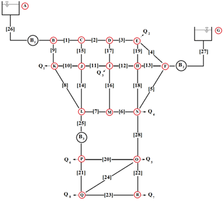
Water flows through a pipe network of pre-stressed reinforced concrete tubes. The absolute roughness, according to ^[2], is 0,04mm. The reservoir "A" is at an elevation of 277 m and reservoir "G" is at an elevation of 330 m. Demand identifiers, demand values, pipe identifiers, pipe diameters, pipe length, node elevation and node identifiers are described on table 5, table 6, table 7. The pumps curves are represented by the equations 2, 3, 4, where HB1, HB2 and HB3 as Pump’s Head [m] and Q as Pump’s Flow [m³/s].

[TeX:] H _B1 = - 158.47Q ² + 55.31Q + 134.20 (2)

[TeX:] H _B2 = -143.65Q ² - 54.78Q + 90.89 (3)

[TeX:] H _B3 = -953.86Q ² + 179.73Q + 47.33 (4)

Table 5 Demand data for Case 03. Source: authors 

Demand Points	Demand [m³/s]
Q1	0,0388
Q2	0,0333
Q3	0,0444
Q4	0,0250
Q5	0,0388
Q6	0,0333
Q7	0,0333
Q8	0,0250

Table 6 Pipe data for case 3. Source: authors 

Tube	D [m]	L [m]	Tube	D [m]	L [m]
1	0,305	457	15	0,152	335
2	0,203	305	16	0,152	366
3	0,254	366	17	0,254	548
4	0,254	610	18	0,152	548
5	0,203	853	19	0,152	396
6	0,203	335	20	0,203	305
7	0,203	305	21	0,203	366
8	0,203	762	22	0,203	335
9	0,203	247	23	0,203	335
10	0,152	396	24	0,152	548
11	0,152	305	25	0,305	457
12	0,152	335	26	0,508	152
13	0,152	305	27	0,508	152
14	0,152	548	28	0,305	762

Table 7 Node data for case 3. Source: authors 

Node	Elevation [m]	Node	Elevation [m]
A	227	J	309
B	301	K	300
C	311	L	308
D	316	M	312
E	322	N	319
F	330	O	330
G	330	P	335
H	320	Q	327
I	314	R	338

Results and Discussion

Evaluation of the methods for the previously described cases.

Case 01

The converged flow values for each method assessed are described on table 8, where it can be seen that no significant differences were found.

Table 8 Converged flow (Q) values [m³/s] and head loss (W) [m], Case 0. Source: authors 

Tube	HC		EPANET		MATLAB
	Q	W	Q	W	Q	W
1	0,1376	5,6249	0,1371	5,6400	0,1376	5,6218
2	0,0626	3,6984	0,0621	3,6840	0,0626	3,6938
3	0,0366	3,6765	0,0365	3,9745	0,0366	3,6801
4	0,1011	3,5712	0,1006	3,5720	0,1011	3,5742
5	0,0261	0,1054	0,0256	0,1040	0,0261	0,1057

In this case, the execution time for all the methods was less than one second, which was considered a fast simulation. Even though the Hardy Cross took 3 times the number of iteration of the Matlab, possibly, because the trust region dogleg technique used by fsolve allows the method to avoid local maximums and minimums accelerating the method convergence.

Case 02

The flow results for each method considered here are described on table 9. The deviation among the methods is no greater than 0.5%. It is noticeable that the accuracy, for this case, may be considered as very good

Table 9 Converged flow (Q) values [m³/s] and head loss (W) [m], Case 02. Source: authors 

Tube	HC		EPANET		MATLAB
	Q	W	Q	W	Q	W
1	0,624	67,4845	0,623	61,7550	0,624	67,4811
2	0,327	18,6270	0,327	14,0971	0,327	18,6213
3	0,189	7,2527	0,189	7,3577	0,189	7,2521
4	0,079	1,1546	0,079	1,1704	0,079	1,1545
5	0,049	5,7452	0,049	0,3843	0,049	5,7467
6	0,109	0,3836	0,109	1,7263	0,109	0,3832
7	0,055	8,1852	0,055	3,2739	0,055	8,1735
8	0,055	1,6210	0,055	1,6283	0,055	1,6188
9	0,297	14,4738	0,297	14,6148	0,297	14,4784
10	0,138	2,6614	0,138	2,7084	0,138	2,6630
11	0,114	3,0028	0,114	3,0528	0,114	3,0033
12	0,183	6,8039	0,182	6,8824	0,182	6,8033
13	0,206	5,7452	0,206	5,8194	0,206	5,7467
14	0,224	5,7110	0,223	5,7297	0,224	5,7107

The execution time was also less than a second. As in the Case 01, the Hardy Cross took 3 times the number of iteration of the Matlab.

Case 03

The converged flow values, for each method evaluated, are described on table 10. The Hardy Cross and Matlab results are in a close agreement with deviations lower than 0.5%. However, there is a clear discrepancy on the EPANET results compared with the other two methods. Differences ranging from 0.1% up to 115% were found. These huge differences are possible due to the same reasons that were described before for Case 01, which means stop criteria on the same order of the flow on the tube, for small number of tubes, while the overall system has converged.

Table 10 Converged flow (Q) values [m³/s] and head loss (W) [m], Case 03. Source: authors 

Tube	HC		EPANET		MATLAB		Tube	HC		EPANET		MATLAB
	Q	W	Q	W	Q	W		Q	W	Q	W	Q	W
1	0,0790	1,3660	0,0599	0,8272	0,0789	1,3656	15	0,0333	6,3175	0,0312	5,6582	0,0333	6,3165
2	0,0456	2,4526	0,0287	1,0431	0,0456	2,4518	16	0,0235	5,3517	0,0228	5,1128	0,0235	5,3513
3	0,0213	0,2383	0,0382	0,7064	0,0213	0,2384	17	0,0669	1,9884	0,0668	2,0167	0,0669	1,9881
4	0,0523	2,0870	0,0665	3,3306	0,0523	2,0867	18	0,0026	0,0958	0,0032	0,1425	0,0026	0,0962
5	0,0232	1,9336	0,0289	2,9684	0,0232	1,9327	19	0,0023	0,0577	0,0050	0,2257	0,0023	0,0579
6	0,0794	7,7318	0,0812	8,2008	0,0794	7,7319	20	0,1003	11,0158	0,0984	10,7787	0,1003	11,0186
7	0,1030	11,5951	0,1040	11,9926	0,1030	11,5649	21	0,0808	8,7304	0,0794	8,5717	0,0808	8,7304
8	0,0708	14,1154	0,0676	13,1369	0,0708	14,1150	22	0,0075	0,9081	0,0065	0,0771	0,0075	0,0982
9	0,0986	8,6383	0,0931	7,8571	0,0986	8,6368	23	0,0409	2,1900	0,0399	2,1273	0,0409	2,1900
10	0,0111	0,9548	0,0134	1,3702	0,0111	0,9546	24	0,0149	2,2881	0,0145	2,2084	0,0149	2,2882
11	0,0184	1,8765	0,0217	2,5986	0,0184	1,8766	25	0,2144	9,1229	0,2111	5,9963	0,2144	9,1227
12	0,0194	2,2844	0,0221	2,9480	0,0194	2,2844	26	0,1776	0,1665	0,1530	0,1277	0,1775	0,1665
13	0,0192	2,0294	0,0238	3,1080	0,0192	2,0289	27	0,0947	0,0519	0,1193	0,0806	0,0947	0,0519
14	0,0406	15,0702	0,0395	14,5056	0,0406	15,0696	28	0,0838	2,5493	0,0805	2,4003	0,0839	2,5500

From the results obtained in cases 01 and 03, it is possible to note that the results with EPANET did not always match with the other two methods here studied. For better insight of the EPANET behavior, on ^[13] was developed a genetic algorithm that was able to identify and account the errors in a hydraulic simulator. The authors evaluated the EPANET, where it was found many incorrect values mainly when the head loss in pipes was 10-4 m or less. For low flow values and/or resistance in tubes, a linear relationship was used instead of the equations of Hazen-Williams, or Darcy-Weisbach, resulting in incorrect results.

In ^[2] it was compared the Distributed Engineering Workstation (DEW) and EPANET models for a case consisting of 58 tubes and 2 reservoirs were evaluated. In this analysis, DEW showed different results compared to EPANET. It happened because both simulators were triggered with their default accuracy, 1x10-3. Then DEW’s accuracy was increased to 1x10-4 and 1x10-6, through this was possible to convergence both models at the same answers and to was possible to conclude that DEW does not have a strict stopping criterion for convergence.

Regarding the accuracy of the standard stop criteria of EPANET in ^[13] it was, carried out three other tests where errors occurred in the solutions. These incorrect solutions occur in situations where the default accuracy of EPANET heads tolerance was inadequate. Then the authors carried out the accuracy correction and obtained the improvement in their results. In the present study, the EPANET’s standard precision is 1x10-3. For the Hardy Cross and fsolve methods, the accuracy has been increased from 1x10-3 to 1x10-6. When the results were compared, no change was noticed. Then the accuracy of EPANET was increased to 1x10-6 without changes in the reported results.

As the results of ^[13] were different for the flow conditions of this work, the main point about EPANET's mistaken results is on its method to solve the mass balance equation. According to ^[19] the method chosen to obtain flow and head loss values was the Hybrid Method, also known as Gradient Method, ^[11]. As it is a hybrid method, the authors used two techniques to solve the basic hydrodynamics equations. For the nonlinear part of equation, the Nodal Newton-Raphson was used in ^[20] and for the linear part by mean of the Modified Conjugate/Incomplete Choleski Factorization algorithm ^[11], thus solving both mass balance equation and energy at same time.

The number of equation is large ^[20], especially when network has lots of elements and components. This situation may lead to a high degree of freedom that may reach to a result that validate the mass balance and, consequently, the converge will occur, although, physically does not correspond in a correct way solution. Reinforcing this idea, ^[18] stated that the nodal formulation of Newton’s method exhibits a relatively slow convergence rate and it is highly sensitive to the starting values, and is unable to handle low resistance lines (mainly short lengths of large diameter tubes). Complementing, was presented in ^[6] another disadvantage of the method that is the lack of optimal convergence in large scale networks. To eliminate this problem, some pipes of the network should be temporarily removed in the analysis procedure. Another disadvantage is the high oscillations to achieve optimal convergence. To decrease the oscillations, the value of the variation of heads at the nodes is reduced by half though this will increase the number of iterations.

In this case, the execution time was close to one second, but due to the higher complexity of this case when compared with the other cases, the Hardy Cross method took 12 times the number of iterations needed to converge if compared to the Matlab code. It occurs due to the Trust Region Dogleg Technique behind fsolve.

Evaluation of the influence from the initial guesses

The analysis of the initial guesses influence was carried out only for Case 03 as it is considered the most complex case. The analysis consists in defining three different conditions to select the unknowns for the initial guess: the first one was to consider that 50% of the average demand was set. It means that the demands on the first initial guess were 50% lower than the average demand previously obtained in the simulation for this case. The second criterion was for 100% (average demand) and the third one was for 150% of this reference value. For each condition, a mass balance was checked. As the network has twenty-eight pipes and sixteen nodes, there are sixteen continuity equations with twelve flow unknowns for being specified to check the mass flow balance. These unknowns were selected firstly by the tubes with the highest head loss, then those with smaller head loss and finally by completely random selection. This selection was based on the previous results of the third case and for all of them the mass balance was satisfied.

In addition, another goal apart from examine the robustness of the Hardy Cross method, was also to test if the tubes with the largest head loss would converge to the smallest number of iterations. This hypothesis is because the tubes that have the biggest head losses are the ones that have the major influence at the system convergence.

The tests of the initial guess were carried out only for the Hardy Cross method because Matlab’s function, fsolve, as previously discussed, has no influence of the initial guess and the EPANET has no option for the user to set it. The “Base” values are described on table 11 with the final flows from the tests of the initial guesses. The “Base” values were taken from the converged result of Case 03 and the 12 imposed values on the three conditions are highlighted at table 11.

Table 11 Test results for the tubes that the head losses were great, small, and the random selection. Source: authors 

Tube	Small Head Losses			High Head Losses			Random			Base
	Demands Average			Demands Average			Demands Average
	150%	100%	50%	150%	100%	50%	150%	100%	50%
1	0,079	0,079	0,079	0,079	0,079	0,079	0,079	0,079	0,079	0,079
2	0,046	0,046	0,046	0,046	0,046	0,046	-0,046	-0,046	-0,046	0,046
3	0,021	0,021	0,021	-0,021	-0,021	-0,021	0,021	0,021	0,021	0,021
4	-0,052	-0,052	0,052	0,052	0,052	0,052	0,052	0,052	0,052	0,052
5	0,023	0,023	0,023	-0,023	-0,023	-0,023	-0,023	-0,023	-0,023	0,023
6	-0,079	-0,079	0,079	-0,079	-0,079	-0,079	-0,079	-0,079	-0,079	-0,079
7	0,103	0,103	0,103	0,103	0,103	0,103	0,103	0,103	0,103	0,103
8	0,071	0,071	0,071	0,071	0,071	0,071	0,071	0,071	0,071	0,071
9	0,099	0,099	0,099	0,099	0,099	0,099	0,099	0,099	0,099	0,099
10	0,011	0,011	0,011	0,011	0,011	0,011	0,011	0,011	0,011	0,011
11	-0,018	-0,018	-0,018	0,018	0,018	0,018	-0,018	-0,018	-0,018	-0,018
12	0,019	0,019	-0,019	0,019	0,019	0,019	-0,019	-0,019	-0,019	0,019
13	0,019	0,019	-0,019	0,019	0,019	0,019	0,019	0,019	0,019	0,019
14	-0,041	-0,041	-0,041	0,041	0,041	0,041	-0,041	-0,041	-0,041	0,041
15	0,033	0,033	0,033	0,033	0,033	0,033	0,033	0,033	0,033	0,033
16	0,024	0,024	-0,024	0,024	0,024	0,024	0,024	0,024	0,024	0,024
17	0,067	0,067	0,067	0,067	0,067	0,067	0,067	0,067	0,067	0,067
18	0,003	0,003	-0,003	-0,003	-0,003	-0,003	-0,003	-0,003	-0,003	-0,003
19	0,002	0,002	0,002	-0,002	-0,002	-0,002	0,002	0,002	0,002	-0,002
20	0,100	0,100	0,100	0,100	0,100	0,100	0,100	0,100	0,100	0,100
21	-0,081	-0,081	-0,081	0,081	0,081	0,081	-0,081	-0,081	-0,081	0,081
22	-0,008	-0,008	-0,008	0,008	0,008	0,008	-0,008	-0,008	-0,008	-0,008
23	-0,041	-0,041	-0,041	0,041	0,041	0,041	-0,041	-0,041	-0,041	0,041
24	-0,015	-0,015	-0,015	-0,015	-0,015	-0,015	0,015	0,015	0,015	-0,015
25	-0,214	-0,214	0,214	0,214	0,214	0,214	0,214	0,214	0,214	0,214
26	0,178	0,178	0,178	0,178	0,178	0,178	0,178	0,178	0,178	0,178
27	-0,095	0,095	0,095	-0,095	-0,095	-0,095	-0,095	0,095	0,095	0,095
28	-0,084	-0,084	0,084	0,084	0,084	0,084	0,084	0,084	0,084	-0,084

From table 11 it is possible to notice that some results do not have the same sign as the Base column (as tube 2 at Random column on table 11, for example). The explanation for that is as the results of the tests were compared only for the third case results, the same mass balance equations used on Case 03 were used on the tests. Within those equations, the initial estimated flow direction is already defined. To perform the test 12 flows values were imposed on these equations and the other 16 values were calculated through then. As these 11 values are identical at each demanded average condition, to validate the mass balance equations some of the remaining ones were required to invert their signal, it means, their flow direction was inverted to validate the mass balance. Better explaining, at the initial estimate the mass balance from some tubes had their flow direction different, comparing the initial estimate from the test and from the Base column. Observing table 11 is realizable that the tests values and the “Base” values are, in modulus, the same. Some of them have contrary signals but it is just because the initial estimate had a different direction; it means that in the end of the iterative processes they have the same direction.

To sum up, the tests of initial flow estimate in relation of modulus value and flow direction are the same as the “Base” column, demonstrating the Hardy Cross robustness.

The resulting flow on each tube had no difference greater than 0.2% if compared to the “Base” column, which means that although the initial guesses were different from the average demand no influence on the results was found, once that the mass balance is verified from the initial guess.

The table 12 shows the number of iterations needed to obtain the converged result. It is clear that fewer iterations were needed for the tubes that had the small head losses, followed by the tubes that were random selected and at last the tubes that had the great head losses. Presenting the opposite idea of the hypothesis that the great head losses tubes are would be the one with less iterations.

Table12 Iteration quantity for each average in each proposal. Source: authors 

	Small Head Losses			Great Head Losses			Random Selection			Base
	Average Demands			Average Demands			Average Demands
	50%	100%	150%	50%	100%	150%	50%	100%	150%
Iteration	75	66	70	82	94	101	68	85	93	88

The Hardy Cross accuracy can be explained by the initial estimates that, judging by the precision and low number of iterations, it can say they were very close to the maximum and minimum global values.

Conclusions

In the present work, a study of three of the most important nonlinear methods used for designing pipe networks was carried out assessing the accuracy and robustness of these methods in calculating the main variables for three different pipes networks.

By the results it could be seen, especially by the third case, that EPANET converged to different results compared to the other methods. fsolve function presented the fastest convergence as expected. Hardy Cross method obtained a great precision and it is robust enough to converge even when the initial estimates have great differences among them, as in 50%, 100% and 150% of the average value of the tested demands. This results allows the Cross method to be used in complex situation.

The hypothesis that the number of iterations would be small where the tubes with the greatest head losses were chosen cannot be proven, as the smaller head losses had the short number of iterations, followed by the random selection and then highest head losses.

References

1.  Cassiolato G, Carvalho E, Caballero J, Ravagnani M. Optimization of water distribution networks using a deterministic approach. Engineering Optimization. 2021; 53(1): 107-124. DOI 10.1080/0305215X.2019.1702980.

2.  Porto RM. Hidráulica Básica. São Carlos/Brazil: EESC-USP; 2006.

3.  Justino J, Nogueira E. Estudo e análise de um sistema de distribuição de água: aplicação do método de Hardy Cross utilizando a Equação universal de Darcy-Weisbach e o método de Hazen-Williams. Rio de Janeiro, Brazil: Cadernos UniFOA (Impresso); 2013. DOI 10.47385/cadunifoa.v8i22.147.

4.  Vieira A. Método iterativo de análise hidráulica e dimensionamento ótimo para programação linear de redes de distribuição de água. Rio de Janeiro-Rj. Brazil. 1980. Accessed in: 02/20/2021. Available in: Available in: https://pantheon.ufrj.br/bitstream/11422/2984/1/154097.pdf;metodos 4.

5.  Wood D, Charles C. Hydraulic network analysis using linear theory. Journal of the Hydraulics Division. 1972; 98(7): DOI 10.1061/JYCEAJ.0003348.

6.  Moosavian N, Jaefarzadeh M. Hydraulic analysis of water supply network using a modified Hardy Cross method. IJE TRANSACTIONS C. 2014; 27(9):1331-1338. DOI 10.5829/idosi.ije.2014.27.09c.02.

7.  Jha K, Misha M. Modified Newton-Raphson technique for integrated object-oriented water pipe network analysis. In: 1^st7.  International WDSA/CCWI 2018 Joint Conference; Kingston, Ontario, Canada: July 23-25, 2018. Accessed in: 03/15/2021. Available in: Available in: https://www.semanticscholar.org/paper/Modified-Newton-Raphson-Technique-for-Integrated-Mishra/5682b94417f5fd0f1383f61ebc7304cd71426d54 7.

8.  Jha K, Misha M. Object-oriented integrated algorithms for efficient water pipe network by modified Hardy Cross technique. Journal of Computational Design and Engineering. 2020; 7(1): 56-64. DOI 10.1093/jcde/qwaa006.

9.  MathWorks: Global Optimization Toolbox User’s Guide. Accessed in 04/10/2021. COPYRIGHT 2004-2013by The MathWorks, Inc. Available in: Available in: http://opencourse.ncyu.edu.tw/ncyu/file.php/30/Global_Optimization_Toolbox-User_Guide.pdf 9.

10.  Britto R, Secchi A, Biscais E. Nova metodologia para cálculo de redes de tubulação com anéis. In: XX Brazilian Congress of Chemical Engineering; Florianópolis, Santa Catarina, Brazil. 2015 DOI 10.5151/chemeng-cobeq2014-1850-17216-137975.

11.  Todini E, Pilat S. A gradient algorithm for the analysis of pipe networks. Computer applications in water supply, vol. 1, System analysis and simulation, edited by: Coubeck, K.B., and Orr, C.H., John Willey & Sons. 1988. 1-20. Accessed in: 04/10/2021. Available in: Available in: https://edoc.tips/download/a-gradient-method-for-the-analysis-of-pipe-networks-pdf-download_pdf 11.

12.  Calixto N. Physical controls in the simulation of hydraulic networks in buildings using EPANET 2.0 software. Journal of Physics. 2020; 012028. DOI 10.1088/1742-6596/1708/1/012028.

13.  Gorev N, Kodzhespirova I, Kovalenko Y, et al. Evolutionary testing of hydraulic simulator functionality. Water Resource Manage. 2011; 25: 1935-1947. DOI 10.1007/s11269-011-9782-5.

14.  Muranho J, Ferreira A, Sousa J, et al. A Convergence issues in the EPANET solver. Procedia Engineering. 2015; 119:700-709. DOI 10.1016/j.proeng.2015.08.923.

15.  Rai R, Lingayat P. Analysis and design of urban water distribution network using Hardy Cross method and EPANET. Singapore: Springer Nature Singapore; 2019. DOI 10.1007/978-981-15-6463-5_33.

16.  Potter M, Wiggert D. Mechanics of Fluids. São Paulo: CENGAGE Learning; 2016.

17.  White FM. Mecânica dos Fluidos. 6th ed. Porto Alegre: AMG Editora Ltda.; 2011.

18.  Altman T, Boulos P. Convergence of Newton method in nonlinear network analysis. Mathematical and Computer Modelling. 1995; 21(4): 35-41. DOI 10.1016/0895-7177(95)00004-L.

19.  Rossman L. EPANET 2 USERS MANUAL. Washington, D.C., U.S.:Environmental Protection Agency. EPA/600/R-00/057; 2000. Accessed in: 03/31/2021. Available in: Available in: https://cfpub.epa.gov/si/si_public_record_report.cfm?Lab=NRMRL&dirEntryId=95662 19.

20.  Brkić D. An improvement of Hardy Cross method applied on looped spatial natural gas distribution networks. Applied Energy. 2009; 86: 1290-1300. DOI 10.1016/j.apenergy.2008.10.005.

Received: January 09, 2021; Accepted: February 21, 2021

^*Autor para la correspondencia: [e-mail]

The authors declare that they have no conflict of interest.

Guilherme da Silva Teixeira. Performed the simulations, developed the MatLab´s script, organized the results, analyzed the data, discussed the results, wrote the original draft, and contributed to the final manuscript.

Guillermo Vilalta Alonso. Involved in planning and supervised the work, analyzed the data, reviewed the original draft, discussed the results and contributed to the final manuscript.

Lourival Jorge Mendes Neto. Conceived of the presented idea, involved in planning and supervised the work, reviewed the original draft, discussed the results and contributed to the final manuscript.