


 Servicios personalizados
 Inglés (pdf)
 Articulo en XML
 Referencias del artículo
 Enviar articulo por email
 Citado por SciELO
  Similares en
SciELO
Similares en
SciELO 
 Permalink
Introduction
Human activity monitoring is applied in different medical and sport areas for the assessment of human functional condition, motor ability, frailty and cognitive disorders. Walking speed can be associated with specific functional impairments and is widely used for quantifying the achievements obtained from the therapeutic and rehabilitation treatments. Moreover, walking speed provides information about personal activity and localization for health care applications(Byun et al., 2019; Kobayashi et al., 2018; Li et al., 2021).
In order to estimate spatial-temporal gait features, for example the walking speed, several algorithms have been described, mainly based on gait patterns recorded with the combination of some electronic devices. For example, in (Steckenrider, Crawford and Zheng, 2021), the use of IMU and GPS (Global Positioning System) for outdoor applications is proposed. Other technologies, such as Wi-Fi (Zhang et al., 2020), RFID technology (Barry et al., 2018) and video-cameras (Mehdizadeh et al., 2021), are more suitable to be applied on indoors environments.
Different studies for gait speed estimation have been carried out in order to achieve less expensive procedures. It means the use of the fewest sensors and the ability to be used in any type of environment. The inverted pendulum model (Allseits et al., 2018; Chen et al., 2011; Byun et al., 2019) has been effectively applied with this purpose. However, on one hand, such proposals are based on theoretical assumptions that use to be significantly apart from the real situation, and, on the other hand, the achieved accuracy that they present are very different. The Kalman filter (Sy, Lovell and Redmond, 2021) has also been applied. In that work, a dynamic gait model is fused with the signal provided by inertial sensors. Nevertheless, the use of biometric data that cannot be accurately obtained and the required implementation of gravity estimation for reducing its effect on the linear acceleration measurement, are disadvantages that must be taken into account whether this algorithm is applied. These algorithms require to handle the difficult inherent to the work with more than one IMU.
Several techniques have been implemented for using only a single IMU. For example, in (Brzostowski, 2018) the Zero Velocity Update (ZUPT) algorithm was proposed in order to estimate the velocity drift and a fusion of accelerometer, gyroscope and magnetometer signals was implemented for orientation estimation. The combination of both algorithms provided the walking speed estimation. Since in that research the direct relationship between IMU’s acceleration and angular velocity signals, taking during a gait course, is not ensured, the adequate effectiveness of the fusion process cannot be guaranteed. Other works propose the application of machine learning techniques. In (Hyeong Jeon and Keun Lee, 2018), the Markov chain was proposed to be applied on the processing of signals from an IMU placed on the foot. That development resulted very effective; however, its implementation requires working with a large number of features, some of them very difficult to obtain. In (Byun et al., 2019), a different application of machine learning algorithm is proposed. In that case, the applied algorithm is based in demographic, biometric and spatial-temporal parameters to estimate walking speed; an IMU placed at the lumbar region was used. The implementation of the direct integration of the vertical acceleration signal, discarding the gravity vector, as well as the fusion of acceleration and angular velocity signals, without assuring the linear relationship between them, does not warrantee to achieve an effective result.
In this work, an application of ANN on gait speed estimation is presented. The novelty resides in the proposed new features, which allow for leading to a very effective performance of the task, which is obtained by means of a single IMU placed at lumbar region.
On inertial sensors limitations
The most of IMU comprise gyroscopes, accelerometers and a magnetometer, which exhibit different disadvantages coming from their work principle; that is why the algorithms that address the processing of the signals must take into account such limitations.
The gyroscope measurements are affected by four noise types: the constant bias, the scale factor, white noise and the bias instability, which affect the results of the direct integration procedure, as well as the application of sensor fusion techniques. The constant bias is a constant angular velocity value provided by the gyroscope when it does not perform any rotational movement. In order to compensate the offset, gyroscope signals obtained during a static acquisition (e.g., placing the gyroscope on a fixed surface) are averaged when the expected angular velocity is null. The scale factor is a consequence of sensor calibration errors that arise during its manufacturing and can be determined as the ratio between the gyroscope measures and the true angular velocity. White noise, produced by thermo-mechanical phenomena, is presented as a sequence of zero-mean uncorrelated random values that fluctuate at a rate much higher than the gyroscope sampling frequency. Its integration leads to a zero-mean random walk process, with a standard deviation that grows with the square root of time. Finally, the bias instability is a stochastic error that indicates how instable the bias of a gyroscope is over a certain period of time (gyroscope drift rate) (Hiller et al., 2019).
The accelerometers provide a measure of the difference between the linear acceleration of the accelerometer block and the earth's gravitational field vector. In linear acceleration absence, the accelerometer output is a measure of the rotated gravitational field vector and the device can be used in order to determine the pitch and roll orientation angles. When the accelerometer is not static, the estimation of linear and gravitational acceleration components becomes a problem, yielding to inaccurate estimations of orientation and position (Pak, Fernandez and Dundar, 2018).
Magnetometer sensors measure the magnetic field components, thus, they estimate the orientation with respect to the earth-magnetic field. Such sensors are very useful whenever they do not be working under external magnetic field exposure or close to metallic objects that change the earth-magnetic field (Ghasemi-Moghadam and Homaeinezhad, 2018).
Artificial Neural Network
Artificial Neural Networks (ANN) are inspired in the biologic neural network sin the brain. ANN have been used in order to solve problems in the fields of pattern recognition, clustering and classification (Abiodun et al., 2018). An example of ANN architecture is the feed-forward multilayer network with the training algorithm known as backpropagation (Shahid, Rappon and Berta, 2019).
Several techniques can be implemented in order to prevent overfitting in the ANN training process. One of them is the cross-validation procedure, which is a data resampling method applied for assessing the generalization ability of the models. In k-fold cross-validation, the available learning set is partitioned into k disjoint subsets of approximately equal size. Here, “fold” refers to the number of resulting subsets. This partitioning is performed by randomly sampling cases from the learning set without replacement. The model is trained using 𝑘−1 subsets, which, together, represent the training set. Then, the model is applied to the remaining subset, which is denoted as the validation set, and the performance is measured. This procedure is repeated until each of the 𝑘 subsets has served as validation set. The average of the 𝑘 performance measurements on the k validation sets is the cross-validated performance (Berrar, 2019).
Method and materials
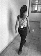
In order to estimate the average gait speed, in this work only one single IMU was placed in the lumbar region, atL3 level. In particular, an IMU BitalinoRIoT (Emmanuel Flety, 2017) was used. This device is based on a 9 DoF LSM9DSO (STMicroelectronics) motion sensor, which includes a triaxial accelerometer (range ± 8 g, sensibility 0.244 mg / LSB), a triaxial gyroscope (range ± 2 gauss, sensibility 0.08 mgauss / LSB) and a magnetometer (range ± 2 gauss, sensibility 0.08 mgauss / LSB). The signals were sampled at 200 Hz. The IMU was fixed at the lumbar region by a velcro tape for achieving a more suitable fixation (see Figure 1).
In addition, the BITalino (r)evolution Plugged platform(Plácido da Silva et al., 2014) was also used in order to implement markers for the initial and final walking times. This allows to compute the true gait speed using the time calculated from the markers and the walking distance fixed for the experiments. Figure 1
A database was built in order to test and validate the technique proposed in this paper. The database comprised the accelerometer and gyroscope signals registered by means of the IMU. Measurements involving 23 healthy subjects, including women and men, with age ranging from 20 years to 50 years, were carried out.
Each subject was asked to walk along a 10 m straight line. Three types of walking were performed: fast, normal, and slow, then, 69 walks were available. Each subject interacted with a button in the Bitalino (r)evolution Plugged for indicating the initial and final walking times.
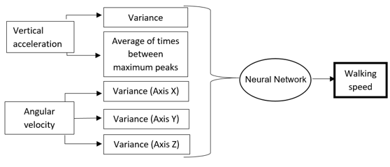
Five features were proposed to be extracted from the signals provided by the IMU: the vertical acceleration variance, the average of times between maximum peaks of vertical acceleration and the three axes angular velocity variances. The vertical acceleration variance was proposed because it was assumed that the amplitude of the acceleration component in this axis and the physical activity involved in the gait process (the gait speed is just a characteristic) are related to some extent. However, the projection of the gravity vector on this axis must be taken into account. Since the trunk could rotate during the gait, a further variation in vertical acceleration may occur that does not correspond to a movement related to the type of gait being executed. That is why, the three axes angular velocity variances are also proposed to work with; these features will represent the variations due to trunk rotations. The average of times between maximum peaks of vertical acceleration was also a chosen feature because it could provide additional information about the gait dynamics.
A feed-forward multilayer network with backpropagation training algorithm was the ANN used in this work for the gait speed estimation. This model is one of the most used neural network in supervised machine learning tasks, whereas the backpropagation algorithm improves the accuracy of predictions in data mining and machine learning. The five features detailed above were used in the ANN training and validation stages (see Figure 2). The feature values were normalized within the range [-1, 1] prior to be given at the ANN input. The activation functions were the hyperbolic tangent sigmoid (hidden layers) function and the linear (output layer) function. The ANN has one output that corresponds with the average gait speed.
Eleven neural network architectures were used to experiment: architectures with either one or two layers and architectures with a number of hidden layer neurons that ranged from 5 to 35. A cross validation (k=3) was implemented in order to select the most effective architecture. The following parameters were used for assessing the effectiveness of the gait speed estimation performed by each architecture:
Absolute error  :
:

Relative error  :
:

RMSE:
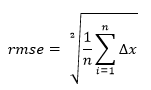
where 𝑥 𝑖 is the estimated gait speed,𝑥 is the true gait speed and𝑛 is the size of test set.
Then, the selected architecture was trained with the 75 % of data, while the rest was used in order to test the trained model.
Results
Firstly, the effectiveness of 11 ANN architectures was evaluated by means of cross validation. The results are shown in Table 1. The notation used in order to make reference to these architectures is the following: number of neurons in the input layer - number of neurons in hidden layer 1 - …- number of neurons in the output layer.
For example, the structure 5-25-1 refers to a feed-forward artificial neural network with five nodes in the input layer, 25 nodes in hidden layer 1 and one node in the output layer. Table 1
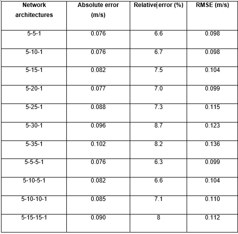
Table 1 reveals that the 5-5-1 network architecture is among the models that achieved the lowest values of absolute error, relative error and RMSE. Therefore, it was the ANN architecture selected for the next stage. This architecture was trained and tested with 52 and 17 feature groups, respectively. Then, the results were compared with those obtained by other algorithms.
True and estimated gait speed for the 17 gait realizations that yielded the test set are shown in Figure 3. The RMSE achieved was equal to 0.08 m/s. The comparison of this result with those obtained by other algorithms is shown in Table 2.
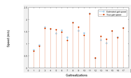
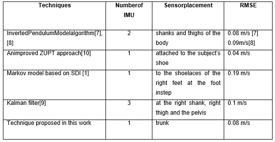
Table 2 shows that the technique proposed in this paper exhibits effectiveness very close to hat obtained by other algorithms. Although ZUPT algorithm exhibits a higher effectiveness, it must be recalled that the foundation of this algorithm does not make clear the relationship between angular velocity and acceleration, which ensure such a high effectiveness. It should be noted that this result was obtained using only one IMU and the five proposed characteristics. Furthermore, this algorithm does not use biometric parameters or the estimation of the gravity vector to compute the gait speed.
Conclusions
In this work, a new algorithm, based on ANN, was proposed to estimate the average gait speed. This proposal resulted as effective as other published proposals. This application does not require the use of biometric parameters or the estimation of the gravity vector; it only uses features extracted from acceleration and angular velocity signals.
In this work, different ANN architectures were evaluated through the computation of parameters RMSE, the absolute error and the relative error. The 5-5-1 was the most effective architecture.
The main contribution of this research was the proposal of new features to estimate the average gait speed: the vertical acceleration variance, the three axes angular velocity variances and the average of times between maximum peaks of the vertical acceleration.

