


 Servicios personalizados
 Inglés (pdf)
 Articulo en XML
 Referencias del artículo
 Enviar articulo por email
 Citado por SciELO
  Similares en
SciELO
Similares en
SciELO 
 Permalink
Introduction
In order to reduce the use of fossil fuels more renewable energy sources (RES), wind and photovoltaic (PV) power, are being used. By the end of 2020 up to 29% of the energy consumed in the world was produced using renewable energy sources. Photovoltaic was the biggest contributor with a growth of over 50%, followed by wind power with a 36% growth [1]. In order to operate a power system correctly, the grid’s frequency must be maintained at a near-constant value. To efficiently control the power system’s operation, the demand’s behavior must be studied as, for example, the load’s peaks and valleys can vary appreciably as seasons change.
Also, workdays and holidays can have very different demand curves. With this information and knowing the number of generators capable of frequency regulation, the upper and lower frequency variation limits can be known. Large frequency deviations can cause stress-producing vibrations in the steam turbines that power electric generators shortening the time between maintenance periods. They may also affect the efficiency of induction motors [2].
Integrating RES, such as wind and PV power, into power systems can cause frequency stability issues. The main challenges rely on their intermittency, variability and uncertainty due to their dependency on weather conditions [3]. As the wind and PV power penetration increases, frequency deviations also increase. If the amount of wind and PV power generation is above the power system’s penetration limit the grid may lose its stability either partially or totally, affecting the quality of the end-consumer service and causing blackouts [4]. In some cases, to avoid a system collapse wind power generation is capped [5, 6]. The integration of RES into power systems are regulated by the grid codes [7].
In order to mitigate frequency stability issues, it is necessary to know the limit of wind and PV generation allowed by the grid. These limits are defined in [8, 9]. This limit can be increased with the introduction of energy storage systems as they can participate in primary frequency regulation as stated in [10, 11]. Frequency deviation analysis is vital for the correct operation of power systems. Several statistic and probabilistic methods, such as Monte Carlo simulations, have been used to analyze frequency deviations. These methods are used to study the variability of wind [12, 13], load variability [14], and the integration of wind power in power systems [15, 16]. An islanded power system is prone to have greater frequency issues than a larger, interconnected power system [17]. Monte Carlo simulations method has also been used to analyze the integration of wind power in isolated power systems [18, 19]. This paper proposes an algorithm based on Monte Carlo simulations to calculate an islanded power system’s wind power limit using frequency deviations as the defining criterion.
Methods and materials
Algorithm used
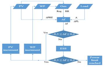
In order to calculate the maximum wind and PV power penetration allowed by the grid it is necessary to consider the characteristics of the wind power and solar power generation as well as the conventional generation characteristics. The algorithm has been divided in subsystems for a better comprehension. First, the system’s load data within a given time frame is introduced. Then the wind power and solar power output data are introduced, and the algorithm continues to calculate the parameters necessary to compute the system’s frequency deviations as well as the maximum solar and wind power penetration allowed by the grid. These parameters include the load-damping coefficient, load variations, wind and solar power variations, the generation distribution and its equivalent regulation.
After the frequency deviation data are calculated the results are compared with the limits set by the grid code. The grid code stablishes that under normal operation conditions frequency values must stay between 59.7 and 60.2 Hz for 95% of the year and between 59 and 61 Hz for 100% of the year. In case frequency deviation values are outside the regulated bounds an energy storage system (ESS) supports the system by providing active power support according to its rated power. If the results comply with the grid code limits, then solar and wind power contributions to the grid are increased and the algorithm is simulated again. If the end results do not comply with the grid code limits, then the last complying values for solar and wind power are set as the maximum power penetration allowed by the power system. The discussed algorithm’s block diagram is depicted in figure 1.
Load model
The load data correspond to hourly measurements within a year’s course and are stored in spreadsheet format. Loads in power systems are comprised of different types. Some are independent from the system’s frequency value, such as resistive loads. Others, such as electric motors, vary their active power as frequency varies in time. According to [20], compound loads can be defined by equation (1):
 (1)
(1)
Where
D |
is the load-damping constant, expressing a load percentage change with respect to a 1% frequency change |
ΔPL |
is the frequency-independent load |
Δf |
is the frequency chang |
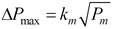
The maximum load variation is calculated using equation (2):
 (2)
(2)
The maximum random variation (ΔPmax) is calculated using km, which relates the mean power (Pm) with the maximum power variation for each load value. Values for km relate to the analyzed time of the year and correspond to values obtained in earlier studies of the analyzed power system [21]. The output of (2) is the maximum load variation corresponding to a given load value. Using this value as limit a Normal distribution is used to obtain random values of load variation smaller than ΔPmax. These values can be positive or negative, corresponding to a load increase or decrease respectively.
Wind farm model
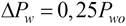
Wind speed is modeled and calculated using Weibull’s distribution using the scale and form factors that correspond to the wind farm site wind speed measurements. The calculated wind speed values are introduced in the wind turbine power curve provided for by the manufacturer resulting in the power output for each wind turbine and subsequently the wind farm. The maximum wind power variation is calculated using equation (3):
 (3)
(3)
Using the output of (3) as limit a Normal distribution is used to obtain random values of wind power variation smaller than ΔP w . These values can be positive or negative, corresponding to a wind power generation increase or decrease respectively.
Photovoltaic farm model
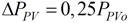
The PV farm power output is modeled using a Normal distribution with its standard parameters calculated corresponding to the site measurements. The farm’s output can be calculated using its power curve taking into account irradiance and cloud cover data at the site. The power curve was built using random values in order to obtain closer-to-reality values. The maximum wind power variation is calculated using equation (4):
 (4)
(4)
Using ΔP PV as limit a Normal distribution is used to obtain random values of solar power variation smaller than ΔP PV These values can be positive or negative, corresponding to a wind power generation increase or decrease respectively.
Generation
In this subsystem the power system’s generation values are calculated in order to obtain the necessary data needed to compute the frequency deviation. The calculation method was developed in [22]. The base of the method is the compliance with the power balance equation shown in equation (5), neglecting power losses and considering the renewables active power as a negative load due to their non-dispatchable characteristics.
 (5)
(5)
A generation dispatch is required to satisfy equation (5). Each generating unit is limited by its designed maximum and minimum power output. These constraints are defined in equation (6).
 (6)
(6)
Where
P i,min |
is the generating unit i minimum output power |
P i,max |
is the generating unit i maximum output power |
NG |
is the amount of generating units in the analyzed power system |
In order to supply the demand (excluding renewables) the sum of the operation costs curves is calculated using equations (7) and (8).
 (7)
(7)
 (8)
(8)
Where Ci is the operation cost of generating unit i. Variables αi, βi, γi correspond to cost constants for generating unit i. After obtaining the generation distribution the algorithm calculates the regulation ranges (RR) for the primary regulation generators. The equivalent regulation (R eq ) is also calculated. Equations (9), (10) and (11), are used to perform these calculations.
 (9)
(9)
 (10)
(10)
 (11)
(11)
According to [21] each generator’s regulation is calculated using equations (12) and (13):
 (12)
(12)
 (13)
(13)
Where
Rpu |
is the per-unit regulation characteristic |
f0 |
is the frequency at no-load |
fn |
is the frequency at rated power |
fB |
the base frequency in Hz |
PB |
the base frequency in MW |
Frequency deviation calculation
After computing the necessary data, frequency deviation (Δf) values are calculated using equations (14) and (15).
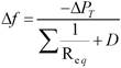 (14)
(14)
 (15)
(15)
At this point in the algorithm, if the regulation range covers any power variations, then equation (14) is used. If power variations are greater than the regulation range, then equation (15) is used instead.
Energy Storage System model
An energy storage system is introduced in the system to support its response to frequency variations in case these are out of bounds. Equation (16).
 (16)
(16)
Where PEES is the energy storage system power output. If the frequency deviations do not comply with the grid code limits then the ESS is used to supply the active power needed in order to keep the frequency within its limits. This operation will be constrained by the ESS rated power. As wind and solar power penetration is increased a possible outcome is that the use of the ESS is not enough to keep the frequency within its designated bounds. In this case the last complying wind and solar power penetration values are established as the maximum allowed by the studied system.
Analysed power system
The studied power system has a radial configuration with five main circuits at 34.5 kV supplying power to the distribution substations. Base generation is provided by four 3.6 MW and four 3.9 MW diesel generators at different geographic locations. In order to maintain quality of service at locations situated far from the main generation sites 1.88 MW generators are installed. These generators also serve as peak power plants at maximum demand.
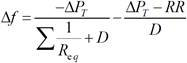
Figure 2, shows the system’s typical daily demand curve for the summer and winter. The winter load curve presents a significant difference between minimum load and maximum load with values of 6.4 MW and 17.8 MW respectively. This difference is much less significant in the summer load curve having a 10.8 MW minimum load and 15.6 MW maximum load.
Another important difference between the summer and winter demand curves is the load ramping, with much faster ramping in the winter. However, since the studied system’s generation is diesel-based, it has a fast enough response so there are no considerable power mismatches between demand and generation. Figure 3, shows how the load is covered per generator type. The base load is covered by the 3.6 MW and the 3.9 MW diesel generators, with the 1.88 MW generators working only in the demand peaks. This load coverage was calculated using an optimization algorithm that is based on an economic pre-dispatch.

The frequency deviation is calculated without any renewables connected to the power system. The frequency deviation histogram is shown in figure 4. The most repeated value was 0 Hz comprising a 21.2% of the total amount. There are 18 out-of-bounds values, representing the 0.02% of the total, corresponding to a correct system behavior as the out-of-bounds values are well below the permitted 5%.

Results and discussion
Among the most important analyzes that must be carried out to verify that the system maintains its frequency within the regulated limits. Being vital the characterization of the system, its regulation, power reserve, and its behavior with different scenarios of integration of renewable sources. To achieve the target of 24% of penetration but maintaining the frequency within the limits established by the Cuban standard.
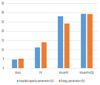
Renewables penetration and emission reduction assessment
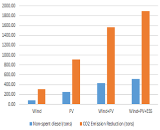
Four study cases with different combinations of renewables, ESS and conventional generation were analyzed. All the scenarios include conventional generation. Figure 5, shows the penetration levels per study case. The lowest penetration values correspond to the wind-only case and the highest value corresponds to the combination of wind, PV and an ESS. As more renewables are installed in the system the fuel consumption is reduced and therefore CO2 emissions are lower. Figure 6, shows the values for the non-spent fuel and CO2 emission reduction per study case.
Conventional generation and wind power
Figure 7, shows that there are two values outside the established limits, representing a 0.27% of the total. The most repeated values are within the limits, with 0 Hz representing a 17.43% of the total. This behavior is considered correct for this system as out of bounds values represent less than 5% of the total.

This scenario deals with the installation a wind power plant in the described power system. The algorithm was run several times resulting in a 1.65 MW wind power plant as the adequate solution.
Conventional generation and solar power
This scenario deals with the installation a solar power plant in the described power system. The most repeated values are within the limits, with 0 Hz representing a 36.9% of the total. Out-of-bounds values represent a 0.46% of the total. Hence the system’s behavior complies with the stablished grid code. This scenario histogram is shown in figure 8.
Conventional generation, wind power and solar power
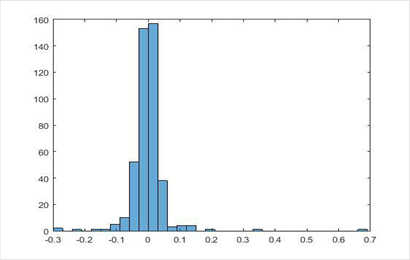
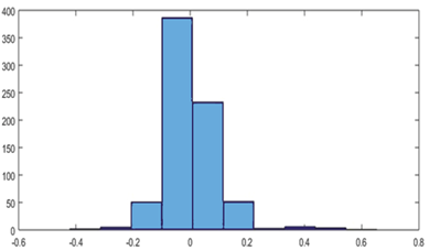
This scenario deals with the installation a solar power plant and a wind power plant in the described power system. The algorithm was run several times resulting in a 4.5 MW wind power plant and a 5.5 MW solar power plant. This scenario histogram is shown in figure 9.
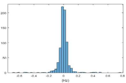
Fig. 9 Frequency deviation histogram for 4.5 MW wind power and 5.5 MW solar power installed capacity
The percentage of frequency deviation values above 0.2 Hz and below -0.3 Hz was 2.42%, below the stablished 5%.
Conventional generation, wind power, solar power and energy storage system
This scenario deals with the installation a solar power plant and a wind power plant in the described power system. The algorithm was run several times resulting in a 5 MW wind power plant, a 5.5 MW solar power plant and a 1 MW energy storage system. The percentage of values within the specified limits is 97.04% with no value above or below 1 Hz. This scenario histogram is shown in figure 10.
Conclusions
A Monte-Carlo-based algorithm was developed to determine the renewable energy sources power limit by calculating the frequency deviations of an isolated power system. The algorithm was run taking into account several scenarios of an isolated power system with different wind and solar power installed capacity values. Conventional generation was considered connected in all scenarios. As expected, frequency deviations increased as the wind and solar power penetration was increased due to the reduction of the conventional generation’s regulation capacity. It was found that when wind and solar work simultaneously, frequency deviations decrease due to the net wind and solar power variations leveling out each other. Also, installing an ESS allowed to increase the system’s renewables power limit due to its capacity to absorb power variations whether it was generating power or using the excess power in the grid to charge itself.
Future works will consider the use of using active power reserve by wind farms. This reserve will be optimized in order to maximize the wind farms energy penetration.

