


 Serviços customizados
 Inglês (pdf)
 Artigo em XML
 Referências do artigo
 Enviar este artigo por email
 Citado por SciELO
  Similares em
SciELO
Similares em
SciELO 
 Permalink
Introduction
Fuel cells work by combining hydrogen and oxygen from the air in an electrochemical process that is clean, quiet and without explosions. Nothing further occurs only electric power, and pure distilled water, together with some heat that can be reused [1].
Some advantages of fuel cells:
No cause environmental pollution.
High efficiency power generation.
Diversity of fuels (natural gas, LP gas, methanol, etc.).
Reuse of heat generated.
Modularity and easy installation.
However, despite having high scores as a source of electrical power, fuel cells have some disadvantages as listed below:
The output voltage varies with the load and with aging.
Have a limited capacity to overload.
Have a slow response to a change in the load, if the fuel supply is adjusted for better efficiency.
Do not absorb any power and can’t accept any curl.
In some technologies are slow at startup.
Fuel cells are considered sensitive or soft voltages sources, because the output voltage has a load dependent nature. The output voltage of a typical fuel cell stack, has a variation of 2-1 no load and full load [2].
Depending on the load connected is required, in the first instance, to design a dc-dc boost converter that accepts a wide range of input voltage, to raise and regulate a higher voltage. The boost converter must have a very fast dynamics to raise the voltage so as to respond more quickly to load changes than the fuel cell; and must be efficient in the conversion process to avoid big losses. Although no ideal converters, should be higher efficiencies than 85%, so that it can be said that the power delivered by the cell is the power received at the load [3].
Power converters contain two main blocks: a power and a control stage. For the power stage design equations of the system according to the requirements of current, voltage, switching frequency, ripple used, etc. to handle. Control is necessary to achieve and maintain power requirements needed in the load. The classic PID control has been widely studied [4,5] and used. The control constants are needed to be adjusted depending on the process to be controlled and remain unchanged for its activity.
DC-DC Converters
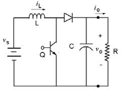
The DC-DC converters are power electronic configurations that allow from a source of constant DC, to control the output voltage DC of the converter [6-8]. These converters have multiple applications: power supplies in computers, distributed power systems, power systems in electric vehicles, etc. The basic settings are three: Buck (reducing), Boost (lift) and Buck-Boost (lift-reducing). These settings allow increase, reduce or increase / decrease the supply voltage (vs) at the output (vo). Each configuration in turn contains four basic elements: inductor (L), capacitor (C), and a controlled switch diode (Q); and the properties of each topology depend on the location of these four elements, see figure 1. It is generally assumed that the charge for the converters is resistive type (R).’
The variable control to regulate the output voltage is controlled switching pattern switch. Being based strategy toggle switch at a fixed frequency varied only time activation thereof: strategy PWM (Pulse Width Modulation). This strategy can be implemented by comparing a saw tooth signal (Vramp) fixed frequency (f) and Vmax peak voltage with a reference voltage (Vref) to achieve the driving voltage (Vpwm), see figure 2, note that you should always meet 0 ≤ Vref ≤ Vmax.
Whereas the DC-DC converters are designed to work under certain operating conditions, it is possible to define the desired output voltage (V0), supply voltage (Vs) and the value of the load resistance, which in the case of would fuel cell output current, and using Ohm's law to obtain the average duty cycle of the converter. However, in reality the converter is subject to various external agents:
Disturbances in supply voltage,
Variations in the load,
Parasitic resistances and voltage drops across the reactive elements of the circuit.
Due to these factors, you should add a control loop so you can regulate the output voltage to the desired value.
Therefore, the problem arises control assuming that the relevant variables have a constant value and a fluctuating part. Equations (1):
Accordingly, it seeks to reduce variations in V0 to the effect of possible disturbances Vs and load resistance, adding a correction factor in the work cycle û(t). This is accomplished using a loop feedback proportional-integral (PI) [7], as shown in figure 3.
The actuator control system (PWM modulator) has the structure shown in figure 4. Its output is then the gate bias voltage (vg) to the active switch Q. Note that the error signal (e) processes the PI controller also represents the variation of the output voltage on your desired average value, emphasizing the control objective is to minimize this variable.
Methodology
Mathematical modeling of the boost converter is performed assuming this works in continuous-conduction mode (CCM), e.g. the current in the inductor and the capacitor voltage have a constant value, and part fluctuating around an average value.
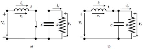
The technique used for the inverter model is based on state space, and define two operating conditions of the active switch Q: ON (μ = 1) and OFF (μ = 0). Then, 2 states are taken in: inductor current iL and the output voltage v0 (which also represents the voltage on the capacitor). Equivalent operating conditions for both circuits are shown in figure 4, note that modes of operation are derived from figure 1.
This way you can get the model of Boost converter: equations (2)
Then obtain an average system whose equations are:equations (3)
where the control variable d = 0 or 1 is the switch status Q. Further, considering that works under a PWM modulation scheme, an average system model taken in equations(3).
The next step should be linearized to (3), since they are found in currently is not possible to apply any transformed, since the system is not linear, so it is considered initial conditions associated with a disturbance as shown in equations (4):
where capital letters indicate the initial conditions and the letters with "^" sign above delimit a small perturbation, such considerations are substituted in equations (5), to obtain the following linearized equations:
To make the association with state space is necessary to make the following change of variables, for further clearing of derivatives in equations (6):
Getting in matrix representation: equations (7):
Now you can get an approximation of the average linear model in terms of the transfer functions equations (8) and equations (9):
The transfer functions equations (8) and equations (9), are stable and show that the poles depend on the condition of the average duty cycle U. Further, equations (8) and equations (9), show a damped response (complex poles) on condition 4R2(1-U)2C-L>0. In addition, we have equations (8), is non-minimum phase because it has an unstable zero (see table 1), which will limit the performance of the control system. The dynamic characteristics of the function G1(s) transfer are shown in table 1.
Components Selection
To choose the necessary components required to know the behavior of the fuel cell so it is necessary to know the polarization curves of the same, and based on these data the following steps to select the appropriate components.
Table 1 Dynamic characteristics of transfer function G1(s) in boost converter.
| Boost | ||
|---|---|---|
| Poles | ωr |
|
| ξ |
|
|
| Zeros |
|
|
| Mr |
|
|
| ωr |
|
Step 1:
From the equation in table 1:
You can get the L/C ratio being:equations (10)
Where ξ is the damping ratio, the load resistance R, D the duty cycle, L the inductance of the inductor and C the capacitance of the capacitor; so desires a configuration in which the oscillatory system is not, so a damping coefficient of 0.5 is established and the capacitor winding ratio is calculated.
Step 2:
A value of inductance that is commercial is selected and the value of the capacitor is calculated based on the ratio L / C or viceversa view equations (10).
Step3:
A working frequency (f) is selected and from the following equations (11) and (12):
Where ΔIL is the variation in the output current, ΔV0 is the variation in the output voltage, Vs is the input voltage and V0 output voltage, substituting the values obtained above in equations (11) and (12) , can estimate which are the variations in the system, if these values are greater than the desired one proceeds to the next step.
Step 4:
Change the value of the frequency (f) on the basis that if the values of ΔIL and ΔV0 are higher than desired, the frequency should increase and repeat the previous step with the new frequency selected.
Design of drivers pi
The designs of the PI controllers are divided into two stages. First the range that can take proportional Kp and integral Ki gains of the controller to maintain stability of closed loop is defined. The controller structure is given by equations (13):
The stability analysis is performed by applying the Routh-Hurwitz criterion [9, 10], the characteristic polynomial of the transfer function T (s): equations (14).
Where S(s) represents the transfer function of sensitivity. The choice of the PI controller is focused on improving the characteristics of tracking control system due to the integral controller action.
It is not considered to include derivative action because it has a high sensitivity to noise in the measurement of voltage sensor.
Stability Analysis Boost Converter
Taking the transfer function equations, as a basis for the stability analysis, obtaining stability margins: equations (15).
Now, it is noted that the proportional gain is limited to its maximum value (1-U) / Vo, this zero due to non-minimum phase of the plant G1 (s).
Results
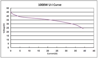
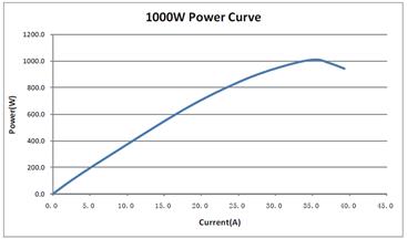
To determine the capacity values for the capacitor (C) and the inductor (L), you must know the device where the converter is used, in this case a fuel cell whose behavior is plotted in the figures below. In which the voltage-current curves (VI), figure 5, and power-current (PI), figure 6, which we can obtain information about the maximum and minimum voltages required by the fuel cell are observed and behavior at the point of maximum power, with which controller design will also, shows some data for certain powers in the fuel cell and operating parameters such as the duty cycle D.
Using step 1 of section 3.1 and relating to table 2, for 1000 W is obtained that L=2.04*C and for 100 W is obtained that L=324*C, so that lesser powers the system tends to be oscillatory, but if L is 324 times greater than C and have greater power 100 W the system would work as an underdamped system.
After completing the steps in section 3.1, the values considered are:
Table 2 Specifications of a stack of fuel cell 1 kw
| Power (W) | Voltage (V) | Current (A) | Load resistance @ 48 V (Ω) | Duty cycle (D) |
|---|---|---|---|---|
| 100 | 40 | 2.5 | 23.04 | 0.1666 |
| 200 | 38.46 | 5.2 | 11.52 | 0.19875 |
| 300 | 37.5 | 8 | 7.68 | 0.21875 |
| 400 | 37.2 | 10.75 | 5.76 | 0.225 |
| 500 | 36.81 | 13.58 | 4.608 | 0.2331 |
| 600 | 36.14 | 16.6 | 3.84 | 0.2471 |
| 700 | 35.71 | 19.6 | 3.291 | 0.256 |
| 800 | 34.18 | 23.4 | 2.88 | 0.2879 |
| 900 | 32.49 | 27.7 | 2.56 | 0.3231 |
| 1000 | 29.76 | 33.6 | 2.304 | 0.38 |
Based on the above values is continued performing simulation using Simulink program and the stability analysis described in Section 4, we can deduce a symmetric interval for the controller gains PI as to maintain stability of closed loop.
Thus were obtained the following ranges:
For practical considerations simulations were performed selecting Kp=0.01 and K=3 values. To which the response was simulated in transferring load when the load requires a power of 1000 W.
Using MATLAB SIMULINK program is possible to determine the behavior of the signal at the output of the controller, where figure 7, shows the behavior of the boost converter by including transfer functions shown above, plus constants PI control before included described, where it can be seen that at high power (1000 W) the system is not disturbed clearly because the need to adjust the system output control is not great, otherwise what is observed in figure 8, where low power (100 W) the system has a greater variation because the control affects the system output attenuating the higher pulse system.
While the result of simulations determines that the behavior of driver output reaches the desired value of 48 V output, and with the help of PI controller may be smoothed slope and the peak of the system is reduced because the the controller decreases somewhat. It can also be seen as part of the function corresponding to equation (8), transfer tends to reduce the error to the controller output.
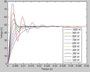
While in figure 9, shows that each which decreases the charging power to boost converter, the system changes from a system critically damped to an underdamped system, because when the system requires less power the given by the duty cycle time is shortened, causing the energy stored in the capacitor is discharged very slowly, so that it stays with or excess voltage causing an overvoltage, but regardless of this time in which it has the surge is very low and the system at the end of 0.05 seconds ends regulated voltage at 48 V desired.
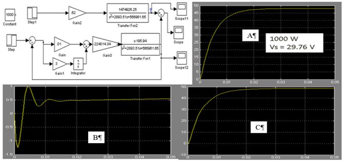
Fig. 7 Simulink diagram obtained with the values of the parameters of the fuel cell operating at a power of 1000 W at the output of the system (A), the output of the PI controller (B) and out of the system without control (C ).
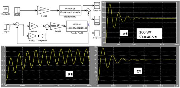
Fig. 8 Simulink diagram obtained with the values of the parameters of the fuel cell operating at a power of 100 W at the output of the system (A), the output of the PI controller (B) and out of the system without control (C ).
Conclusions
By using voltage converters type boost is possible to regulate the voltage of a fuel cell, in addition to following a methodology to find the transfer function of this type of converters also use based control system states you can find such transfer functions, and by the Routh-Hurwitz is possible to find constants for designing a functional PI controller, and can be applied to a system of fuel cell stack with high efficiency in energy conversion and especially to maintain a nearly constant voltage of 48 V, coupled surge suppressor system, which can be connected to an inverter, and that it has no power fluctuations that prevent an electrical charge that requires power from 100 to 1000 W.

