


 Serviços customizados
 Inglês (pdf)
 Artigo em XML
 Referências do artigo
 Enviar este artigo por email
 Citado por SciELO
  Similares em
SciELO
Similares em
SciELO 
 Permalink
Introduction
During the last 25 years, the Zeolite Engineering Laboratory of the Materials Science and Technology Institute of the University of Havana has focused its research on the design and development of new materials based on natural zeolites (NZ). These materials have been used to obtain high value-added products with applications in different branches of industry, especially those linked to the pharmaceutical sector. An example of this are the NZ modified with Cu or Zn that have microbicidal properties related to the oligo dynamic activity of the exchanged elements.
The NZ belonging to the Tasajera deposit meets the requirements established in the Cuban Standard 625 of 2008 1 for its use in the Cuban pharmaceutical industry. The analytical control of the exchanged element is of vital importance since it conditions the possible use of the material. To carry out this control, consolidated analytical techniques such as flame atomic absorption spectrometry (FAAS) and inductively coupled plasma optical emission spectrometry (ICP-OES) are used. Although with these techniques it is possible to obtain unbiased results with good precision, they require the dissolution of the sample prior to analysis, an extremely cumbersome process that involves a considerable consumption of time and chemical reagents.
Contrary to this, energy dispersive X-Ray fluorescence (EDXRF) is an analytical technique that has the advantage of presenting the sample to the instrument in solid phase, either in the form of loose powder or in briquettes of different sizes and thicknesses. In addition, it allows the determination of major and minor elements in diverse matrices in a precise and exact way. On the other hand, EDXRF is a non-destructive and environmentally friendly technique since it does not generate waste.
The objective of this work is to develop an analytical procedure by EDXRF in order to obtain reliable results of the Cu and Zn content in the modified NZ produced in the Zeolite Engineering Laboratory of the Materials Science and Technology Institute of the University of Havana. To achieve the above, it is necessary to validate the procedure and thus offer documented evidence that demonstrates that it is suitable to be used for that purpose.2
It is known that there are a large number of sources 3-5 that provide general indications regarding how the validation of an analytical procedure should be carried out. However, there is no general consensus regarding the performance parameters of the procedure to be taken into account in the validation, so the diversity of terms and criteria prevails.6 However, those with the greatest incidence on the reliability of the result are the precision, the bias and the combined uncertainty of the measurement. The last performance characteristic is very important because of its great influence on the decisions that can be made with the result. For this reason, it is now required that all testing laboratories issue their results accompanied by the combined uncertainty of the measurement.7 Validation of an analytical procedure is not considered complete without estimation of this performance characteristic.
Materials and methods
Preparation of reference materials
The reference materials were prepared by weighing known amounts of NZ from the Tasajera deposit with CuSO45H2O (ZN-Cu) orZnSO47H2O (ZN-Zn) in a porcelain capsule. Subsequently, a small portion of deionized water was added and gently stirred with an agate pestle for 3 min. The mixture was dried at 100 oC in an oven and after cooling to room temperature it was homogenized for 5 min.
The contents of Cu and Zn expressed as a mass fraction in percent mass/mass in the reference materials were estimated according to:
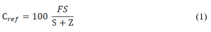
where S is the weighed mass of CuSO45H2O or ZnSO47H2O,Zthe weighed mass of NZ and F is the ratio of atomic masses (gravimetric factor) of each element in its respective hydrated salt. The combined uncertainty (uref) associated with the Cref concentration value was estimated as established in the Guide for the Expression of Uncertainty in Measurement (GUM).8
Samples reference preparation for FAAS measurement
The determinations were carried out on the samples selected for validation. About 0,1 g of each sample was weighed on graphite crucibles of 125 mL capacity. Then, 5 mL of 40 % HF were added, keeping the crucibles covered and at rest for 24 h. Once that time had elapsed, 1 mL of 60 % HClO4 was added and heated on an electric hot plate until dense white fumes appeared. The contents of the crucibles were allowed to cool, 3 mL of 40 % HF was added, and heating was repeated until dense fumes. Subsequently, the walls of each crucible were washed with a fine stream of deionized water, 3 mL of 37 % HCl was added and heated until the sample dissolved. The crucibles were allowed to cooland the dissolved samples were transferred to a volumetric flask with a capacity of 100 mL. All reagents used were of analytical purity.
Instrumental conditions for FAAS spectrometer
Measurements were made in a Shimatzu model AA-6800 atomic absorption spectrometer operated under the instrumental conditions that appear in table 1.
Preparation of tablets for measurement by EDXRF
0,5 g of H3BO3 and 1 g of modified zeolite sample were weighed out separately. The solids were transferred in that order to a stainless steel die in individual layers as homogeneously as possible. Finally, the die was placed in a hydraulic press and a pressure of 15 MPa was applied.
Instrumental conditions for EDXRF spectrometer
EDXRF measurements were performed on an Oxford Instruments energy dispersive X-Ray spectrometer model X-Supreme. This equipment consists of an SDD-type Si semiconductor detector with a resolution of 169 eV for Zn Kα and a 3-watt X-Ray tube with W anode. In addition, it has three types of primary radiation filters and offers the possibility of working in atmospheres of He and air.
Table 2 shows the measurement conditions under which all the spectra were recorded. The values (keV) corresponding to the maximum of the analytical line Kα of the elements Cu and Zn and the lower and upper limits of the region of the spectrum around these maximums where the measurement of the area of the signal in counts per second (cps) were carried out are also shown.
Table 2 Instrumental conditions of measurement by EDXRF. The values for Cu and
| Measurement condition | Value | |||
|---|---|---|---|---|
| Applied voltage to x ray tube (KV) | 20 | |||
| Applied current to the x ray tube (µA) | 100 | |||
| Radiation primary filter | W (5µm thickness) | |||
| Acquisition time of the spectrum (s) | 120 | |||
| Atmosphere | Air | |||
| Sample adaptor | Cd | |||
| Element | Maximum | Lower limit | Upper limit | |
| Cu | 8,04 | 7,85 | 8,24 | |
| Zn | 8,63 | 8,50 | 8,80 | |
Procedure validation
The validation of the analytical procedure included the estimation of the following performance characteristic: bias (Δ), scope, combined measurement uncertainty (uc), precision in repeatability conditions (Sr), in intermediate conditions different analyst (SiA), different time (SiT) and different time-analyst (SiTA).
The precision, bias and uncertainty of the measurement were estimated at five concentration levels defined by the reference samples selected for validation. For this purpose, a validation experiment applied to each element was carried out.
The validation experiment is a fully nested three-factor design according to the ISO 5725-39 standard. It was structured as follows: on D non-consecutive days (Factor 1) A analyst (Factor 2) made N determinations under repeatability conditions (Factor 3) of the Cu and Zn content by EDXRF in the corresponding reference sample.
Estimation of performance characteristics
Precision
The different precision estimates were obtained from the sums of squares and mean squares due to each factor in the nested design according to:


where:
SSR, SSA, and SSD are the sums of squares due to the repeatability, analyst and day factors, respectively.
CMR, CMA and CMD are the respective mean squares.
D, A and N are the number of days, the number of analysts and the number of replicates made by each analyst, respectively.
Sr 2, SA 2 and ST 2 are the variances of repeatability, analysts and days, respectively.
Bias
The estimation of the bias and its associated uncertainty was carried out using two totally different procedures. The first is based on estimating the recovered:
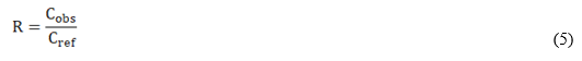
and then the statistician t:
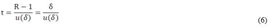
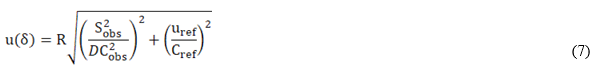
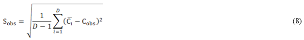
where C i is the average of the results obtained by the A analysts on each day, Cobs is the average of C i and constitutes the concentration value (%) estimated by EDXRF in the corresponding reference sample. The term δ is the bias in terms of recovery and u(δ) its associated uncertainty which was estimated according to Barwick and Ellison10, Cref is the concentration of the reference sample and uref its uncertainty.
The value of the t-statistician obtained from equation (6) is compared with the critical values of the Student's t-distribution. If it is true that t1-α⁄2; D-1 ≤ t ≤ t1 - α⁄2; D-1, the bias is not statistically significant for the selected confidence level α.
The second method is based on the comparison of the concentrations obtained by EDXRF in the reference samples (Cobs) with the corresponding concentration values obtained by FAAS (CFAAS) according to:

The values of the intercept a and the slope b were estimated by linear regression using the Iteratively Reweighted Least Squares (IRLS) method11. The bias evaluation was carried out from the joint estimation of the significance of the intercept and the slope by mean of its confidence ellipse.12 The test result is best visualized as a plot of intercept vs. slope where the point (a, b) and the confidence ellipse are represented. If the point (a= 0, b= 1) is inside the ellipse, the bias of the EDXRF procedure is not statistically significant.
Combined measurement uncertainty
The combined measurement uncertainty was estimated according to:

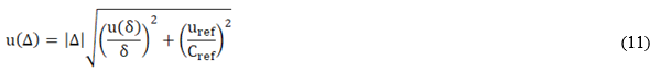
where ∆= Cref δ is the bias and u(Δ) is its associated uncertainty, both expressed in % mass/mass.
Scope
From four NZ samples belonging to deposits different from Tasajera, twelve reference materials were prepared (three for each sample) following the procedure described above. The differences in the content of SiO2 in these samples with respect to that of the zeolite from the Tasajera deposit (60-68 %) was used as the main criterion for selection. The content of SiO2 of such samples appears in table 3.
Results and discussion
Table 4 shows the concentrations of Cu and Zn (Cref) calculated using equation (1) for the reference materials prepared from the NZ belonging to the Tasajera deposit. The combined uncertainties (uref) associated with these concentration values are included in the table. The first seven materials (P1 to P7) that appear for each element were used as calibration standards and the remaining ones (R1 to R5) as reference samples for the respective nested designs.
The tablets that were prepared according to the procedure described were resistant to handling, with well-defined faces and edges. This result rules out the use of binders, which implies weighing this and the reference material on an analytical balance and the exhaustive homogenization of the mixture of both. On the other hand, it would increase the time of the preparation being this more critical if it is necessary to analyze a large number of samples.
Table 4 Cu and Zn contents (Cref) and associated combined uncertainties (uref) in the
| Cu | Zn | ||||
|---|---|---|---|---|---|
| Name | Cref | uref | Name | Cref | uref |
| ZNCuP1 | 0,19 | 0,03 | ZNZnP1 | 0,39 | 0,02 |
| ZNCuP2 | 0,40 | 0,03 | ZNZnP2 | 0,78 | 0,02 |
| ZNCuP3 | 0,99 | 0,03 | ZNZnP3 | 0,97 | 0,03 |
| ZNCuP4 | 1,50 | 0,03 | ZNZnP4 | 1,87 | 0,03 |
| ZNCuP5 | 2,00 | 0,03 | ZNZnP5 | 2,72 | 0,03 |
| ZNCuP6 | 2,52 | 0,03 | ZNZnP6 | 3,52 | 0,03 |
| ZNCuP7 | 4,83 | 0,03 | ZNZnP7 | 4,27 | 0,03 |
| ZNCuR1 | 0,80 | 0,01 | ZNZnR1 | 0,48 | 0,01 |
| ZNCuR2 | 1,19 | 0,01 | ZNZnR2 | 1,00 | 0,01 |
| ZNCuR3 | 1,79 | 0,01 | ZNZnR3 | 2,00 | 0,01 |
| ZNCuR4 | 2,18 | 0,01 | ZNZnR4 | 3,00 | 0,01 |
| ZNCuR5 | 4,80 | 0,02 | ZNZnR5 | 4,00 | 0,01 |
The selected measurement conditions (table 2) allowed the detector dead time in all measurements to be less than 20 % (manufacturer's recommendation). The use of the W filter considerably reduces the background and practically eliminates the W Lα line (8,39 KeV). This line belongs to the X-Ray tube and is scattered by the sample. If it appears in the spectrum, it constitutes a potential interference to the Kα of Zn (8,63 KeV). The spectrum acquisition time ensured that the relative standard deviation (RSD) of the analytical signal area was less than 1 %. The RSD was estimated according to:

where T is the acquisition time of the spectrum and A is the area under the analytical signal defined by the counts per second accumulated in the region of interest.
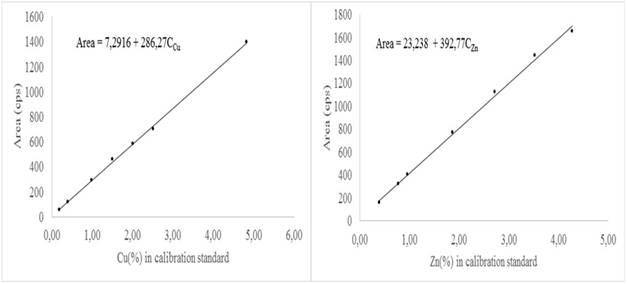
Estimation of the concentration in the validation samples
Figure 1 is the calibration curves for Cu and Zn in one of the days of execution of the nested design. As can be seen, the behavior of the area of the analytical signal with respect to the concentration of Cu or Zn in the respective calibration standard is linear. This is an indication that the matrix does not exert any absorption or enhancement effect in the signal of both elements.
This behavior was observed for all the calibration curves obtained. Thus, the calibration function Area = I + PC was used to model this behavior. The values of the intercept I and the slope P were estimated by ordinary least squares. This calibration function was used to calculate by analytical interpolation the content of Cu and Zn in the samples selected for validation.
Estimation of performance characteristics
Precision
Table 5 shows the results of the estimation of precision (%, mass/mass) in repeatability conditions (Sr), intermediate conditions different analyst (SiA), intermediate conditions different time (SiT) and intermediate conditions different time-analyst (SiTA). The analyst standard deviation (SA) and the time standard deviation (ST) also appear.
These values were obtained by applying equations (2-4) to the results of the nested design where 3 analysts carried out on 4 non-consecutive days 2 determinations in repeatibity conditions of Cu and Zn content in the corresponding reference samples.
Table 5- Results of the precision estimates for the EDXRF procedure. All the results
| Zn | ||||||
|---|---|---|---|---|---|---|
| Cobs | Sr | SA | ST | SiA | SiT | SiTA |
| 0,49 | 0,011 | 0,013 | 0,006 | 0,017 | 0,013 | 0,019 |
| 0,99 | 0,023 | 0,015 | 0,014 | 0,028 | 0,027 | 0,031 |
| 1,99 | 0,047 | 0,042 | 0,056 | 0,063 | 0,056 | 0,070 |
| 3,00 | 0,080 | 0,043 | 0,089 | 0,091 | 0,120 | 0,127 |
| 3,99 | 0,125 | 0,102 | 0,151 | 0,162 | 0,149 | 0,180 |
| Cu | ||||||
| Cobs | Sr | SA | ST | SiA | SiT | SiTA |
| 0,82 | 0,013 | 0,012 | 0,006 | 0,018 | 0,014 | 0,019 |
| 1,22 | 0,018 | 0,017 | 0,019 | 0,025 | 0,026 | 0,031 |
| 1,81 | 0,023 | 0,027 | 0,017 | 0,035 | 0,028 | 0,039 |
| 2,20 | 0,027 | 0,037 | 0,032 | 0,045 | 0,041 | 0,055 |
| 4,86 | 0,074 | 0,038 | 0,074 | 0,083 | 0,104 | 0,111 |
The ISO 5725-613 standard establishes that in routine tasks the control of precision in repeatability conditions of the analytical procedure should be carried out by means of the maximum permissible deviation between replicates (MPD):

where T0,95,n is a tabulated value that appears in the standard for different number of replicates n and 95 % confidence level. For n = 2, a value widely used in routine, the MPD = 2,8Sr. However, if the average of the replicates does not coincide with some concentration value of the validation samples, then it is necessary to use the so-called characteristic function14 to estimate the corresponding Sr and therefore the MPD.
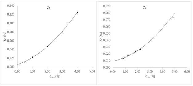
The characteristic function models the behavior of Sr with concentration and figure 2 is a graphical representation of that behavior. As can be seen, in both elements the increase in Sr with the increase in Cobs shows a non-linear trend. Thus, using the values of Cobs and Sr that appear in table 5, the respective characteristic function was obtained for Cu and Zn:


In routine tasks, the above equations allow the estimation of Sr for sample concentrations (obtained as an average of replicates) that do not coincide with the Cobs of the validation samples. In this way, it is possible to have the corresponding DMP and carry out the precision control as established by the aforementioned ISO 5725-6 standard.
Bias
The results obtained in the evaluation of the significance of the bias through the recovery are shown in table 6. In it, the tabulated values for the recovery R, the bias δ, its uncertainty u(δ) and the value of the statistician t were obtained from equations (5-8). As can be seen, for both elements the t-statistician is between the limits established by the critical values of the Student's t-distribution for 95 % confidence and 3 degrees of freedom (D-1). Therefore, it can be stated with this level of confidence that there is no statistical evidence to affirm that the bias is significant, that is, it is accepted that there is no systematic error.
Table 6 Results of the bias evaluation through the recovery
| Zn | |||||||
|---|---|---|---|---|---|---|---|
| Cref | Cobs | R | δ | u(δ) | t | -t0,975,3 | t0,975,3 |
| 0,49 | 0,49 | 1,00 | 0,004 | 0,04 | 0,08 | -3,18 | 3,18 |
| 1,00 | 1,00 | 1,00 | -0,003 | 0,02 | -0,16 | ||
| 2,00 | 1,99 | 0,99 | -0,007 | 0,01 | -0,63 | ||
| 3,00 | 2,98 | 0,99 | -0,007 | 0,02 | -0,31 | ||
| 4,00 | 3,97 | 0,99 | -0,008 | 0,01 | -0,71 | ||
| Cu | |||||||
| Cref | Cobs | R | δ | u(δ) | t | -t0,975,3 | t0,975,3 |
| 0,82 | 0,82 | 1,00 | 0,005 | 0,03 | 0,15 | -3,18 | 3,18 |
| 1,19 | 1,22 | 1,02 | 0,021 | 0,02 | 0,91 | ||
| 1,79 | 1,81 | 1,01 | 0,010 | 0,01 | 0,69 | ||
| 2,18 | 2,20 | 1,01 | 0,011 | 0,02 | 0,69 | ||
| 4,80 | 4,86 | 1,01 | 0,012 | 0,01 | 0,91 | ||
Although CuSO45H2O and ZnSO47H2O meet the requirement to be considered as reference materials of the composition, the possibility of changes in their structure during the preparation process of the reference materials according to the described procedure cannot be ruled out. This can influence the concentration values of the reference materials and therefore the results obtained with the EDXRFprocedure. For this reason, the estimation and evaluation of bias by regression was decided.
Table 7 shows the contents of Zn and Cu determined by FAAS in the reference samples selected for validation as well as the combined uncertainties associated with these concentration values u(FAAS) estimated according to GUM8. These contents are the average of 3 replicates carried out by two analysts under repeatability conditions. The results obtained by EDXRF (Cobs) and its uncertainty Sr (values taken from table 5) are also included.
Table 7 Results of the determinations by FAAS and EDXRF (C obs) in the samples selected for validation. All the tabulated values are in % mass/mass
| Zn | Cu | ||||||
|---|---|---|---|---|---|---|---|
| Cobs | Sr | FAAS | u(FAAS) | Cobs | Sr | FAAS | u(FAAS) |
| 0,49 | 0,011 | 0,44 | 0,02 | 0,82 | 0,013 | 0,89 | 0,02 |
| 1,00 | 0,023 | 0,94 | 0,03 | 1,22 | 0,018 | 1,17 | 0,01 |
| 1,99 | 0,047 | 2,06 | 0,04 | 1,81 | 0,023 | 1,84 | 0,03 |
| 2,98 | 0,080 | 2,95 | 0,06 | 2,20 | 0,027 | 2,33 | 0,03 |
| 3,97 | 0,125 | 4,02 | 0,08 | 4,86 | 0,074 | 4,98 | 0,03 |
Figure 3 is a graphic representation of the estimated concentrations of Zn and Cu in the reference samples by EDXFR (Cobs) and FAAS. The figure also shows the result of the linear regressions by IRLS.
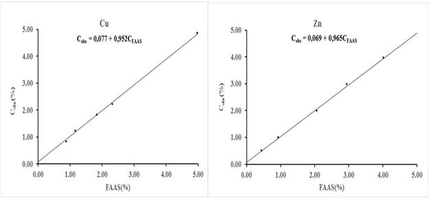
Fig. 3 Behavior of the results of Zn and Cu determination by FAAS in the reference samples with respect to the obtained in the same ones by EDXRF. The value of the intercept and slope of the equations in the graphic were estimated by IRLS regression
The FAAS is an analytical technique with chemical-physical fundamentals completely different from those of the EDXRF. The way the sample is presented to the instrument is also totally different. Consequently, if the intercept and slope of the linear equations that appear in figure 3 are not statistically different from zero and one, respectively, it is possible to affirm that the bias of the EDXRF procedure is not significant in the validation interval. IRLS regression was used because it considers the uncertainties associated with the results of the two methods in estimating the intercept and slope.
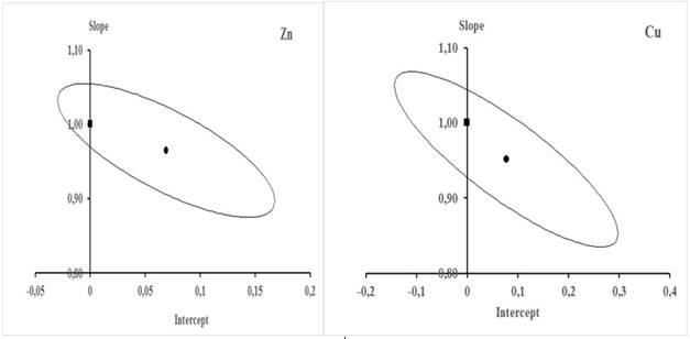
Fig. 4 Joint 95 % confidence interval (ellipse) of the intercept and slope (circle) belonging to the equations showed in figure 3. Thesquare represents the values intercept = 0 and slope =1
Figure 4 shows the results of the joint significance test of the intercept and slope estimated by IRLS. The confidence level of the test was 95 %. As can be seen in the figure, the point (0,1); represented by a square, is within the ellipse that describes the joint 95 % confidence interval of the intercept and slope (circle). Therefore, it can be stated with this level of confidence that there is no statistical evidence to affirm that the bias of the procedure by EDXRF is significant. This test has the advantage that it includes the covariance between the intercept and the slope.
Estimation of bias using any type of linear regression allows its significance to be assessed globally over a concentration range. In addition, it is possible to know the type of bias if it is significant11. However, it is not possible to estimate the bias (ΔR) and its uncertainty u(ΔR) individually for each of the concentrations in the interval. Borges and collaborators15 offer a way to estimate ΔR and u(ΔR) in this case:

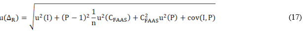
Table 8 Results (% mass/mass) of the estimation of bias ΔR and the associated uncertainty u(ΔR) for the EDXRF procedure. The values of u(Δ) are showed for comparison purposes
| Cu | |||||
|---|---|---|---|---|---|
| Cobs | FAAS | u(FAAS) | ΔR | u(ΔR) | u(Δ) |
| 0,82 | 0,86 | 0,02 | -0,04 | 0,053 | 0,024 |
| 1,22 | 1,15 | 0,01 | 0,07 | 0,060 | 0,028 |
| 1,81 | 1,82 | 0,03 | -0,01 | 0,080 | 0,026 |
| 2,20 | 2,32 | 0,03 | -0,12 | 0,096 | 0,036 |
| 4,86 | 4,98 | 0,03 | -0,12 | 0,191 | 0,062 |
| Zn | |||||
| Cobs | FAAS | u(FAAS) | ΔR | u(ΔR) | u(Δ) |
| 0,49 | 0,44 | 0,02 | 0,05 | 0,043 | 0,021 |
| 1,00 | 0,94 | 0,03 | 0,06 | 0,047 | 0,021 |
| 1,99 | 2,06 | 0,04 | -0,07 | 0,061 | 0,023 |
| 2,98 | 2,95 | 0,06 | 0,03 | 0,076 | 0,071 |
| 3,97 | 4,02 | 0,08 | -0,05 | 0,096 | 0,045 |
In table 8 it can be seen that for both elements u(ΔR) is always numerically greater than u(Δ) and the difference between both tends to increase with the increase in Cobs. If equations (11) and (17) are compared, it is clear that four uncertainty components are involved in the estimation of u(ΔR), while only two are involved in the estimation of u(Δ). In the case of u(ΔR) the dominant components are those of the intercept, slope and covariance, however, for u(Δ) the contribution due to the reference material is practically negligible. In addition, u(Δ) is obtained from a nested experiment in which 24 replicates were made under repeatability conditions, while u(ΔR) is obtained from a regression with only five values.
Combined measurement uncertainty
Table 9 Results of the estimation of the combined measurement uncertainty for the determination of Cu and Zn by EDXRF. All the tabulated values in % (m/m)
| Zn | |||
|---|---|---|---|
| Cobs | SiTA | u(Δ) | u(Cobs) |
| 0,49 | 0,018 | 0,021 | 0,03 |
| 0,99 | 0,031 | 0,021 | 0,04 |
| 1,99 | 0,070 | 0,023 | 0,07 |
| 3,00 | 0,127 | 0,071 | 0,15 |
| 3,99 | 0,180 | 0,045 | 0,19 |
| Cu | |||
| Cobs | SiTA | u(Δ) | u(Cobs) |
| 0,82 | 0,019 | 0,024 | 0,03 |
| 1,22 | 0,031 | 0,028 | 0,04 |
| 1,81 | 0,039 | 0,026 | 0,05 |
| 2,20 | 0,055 | 0,036 | 0,07 |
| 4,86 | 0,111 | 0,062 | 0,13 |
Table 9 reproduces the results of the estimation with equation (10) of the combined measurement uncertainty u(Cobs) associated to the Cobs concentration obtained by EDXRF in the reference samples selected for validation. Values of the uncertainty of the estimation of the bias u(Δ) from the recovery are also shown.
In routine tasks is possible that an estimated concentration (Cest) of Cu or Zn does not coincide with some concentration of the validation interval (Cobs). In order to estimate the combined uncertainty of the measurement associated with Cest, it is necessary to obtain first the so-called uncertainty function16. This function describes the performance of an analytical procedure in terms of the behavior of the uncertainty in a concentration range. Furthermore, it is very useful when it is necessary to compare the value of Cest with a specification limit.17
From the data in table 9, the behavior of u(Cobs) with respect to Cobs was modeled for each element. Figure 5 is a graphical representation of that behavior.
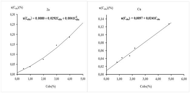
Fig. 5 Behavior of u(Cobs) with respect to Cobs in the validation interval. The equations showed in the figure are the respective characteristic functions
In the case of Cu, it is observed that as Cobs increases the value of u(Cobs) increases linearly, while in Zn the increase of u(Cobs) with the increase of Cobs is parabolic. Figure 5 shows the respective functions that describe these behaviors and allow the estimation for each element of the combined uncertainty associated with any concentration value within the validation interval.
Scope
Table 10 shows the contents (C) of Cu and Zn estimated by EDXRF in the reference samples prepared with natural zeolites that not belong to Tasajera deposit. The corresponding combined uncertainty (uc) and expanded uncertainty (U) values are also shown, as well as the lower (LL) and upper (UL) limits of the coverage interval where 95 % of the values attributable to the concentration C are found. The concentration values of the reference samples (CREF) were obtained from equation (1) and their uncertainties (uREF) according to GUM8.
The concentrations of these samples are at the extremes and center of the concentration range of the reference samples used in the validation. The values of uc in table 10 were obtained from the respective uncertainty functions that appear in figure 5. The expanded uncertainty was obtained as U = 2uc while the limits of the 95 % coverage interval as LL =C - U and UL = C + U. The value of Z was estimated according to:

Table 10 Results of the Cu and Zn estimation in the reference samples prepared with natural zeolites that not belong to Tasajeradeposit
| Cu | ||||||||
|---|---|---|---|---|---|---|---|---|
| Name | C | uc | U | LL | UL | CREF | uREF | Z |
| Z7CuR1 | 0,63 | 0,02 | 0,05 | 0,58 | 0,68 | 0,80 | 0,01 | -6,1 |
| Z7CuR2 | 1,46 | 0,04 | 0,09 | 1,37 | 1,55 | 1,80 | 0,01 | -7,2 |
| Z7CuR3 | 3,29 | 0,09 | 0,18 | 3,11 | 3,47 | 4,02 | 0,02 | -8,1 |
| Z25CuR1 | 0,67 | 0,03 | 0,05 | 0,62 | 0,72 | 0,80 | 0,01 | -4,5 |
| Z25CuR2 | 1,49 | 0,05 | 0,09 | 1,40 | 1,58 | 1,80 | 0,01 | -6,5 |
| Z25CuR3 | 3,31 | 0,09 | 0,18 | 3,13 | 3,49 | 4,01 | 0,02 | -7,7 |
| Z29CuR1 | 0,66 | 0,03 | 0,05 | 0,61 | 0,71 | 0,80 | 0,01 | -4,8 |
| Z29CuR2 | 1,55 | 0,05 | 0,09 | 1,46 | 1,64 | 1,81 | 0,01 | -5,3 |
| Z29CuR3 | 3,50 | 0,09 | 0,19 | 3,31 | 3,69 | 4,00 | 0,02 | -5,2 |
| Z32CuR1 | 0,74 | 0,03 | 0,06 | 0,68 | 0,80 | 0,80 | 0,01 | -2,0 |
| Z32CuR2 | 1,76 | 0,05 | 0,10 | 1,66 | 1,86 | 1,80 | 0,01 | -0,7 |
| Z32CuR3 | 4,04 | 0,11 | 0,21 | 3,83 | 4,25 | 4,00 | 0,02 | 0,4 |
| Zn | ||||||||
| Name | C | uc | U | LL | UL | CREF | uREF | Z |
| Z7ZnR1 | 0,44 | 0,02 | 0,04 | 0,40 | 0,48 | 0,51 | 0,01 | -2,8 |
| Z7ZnR2 | 1,70 | 0,07 | 0,14 | 1,56 | 1,84 | 1,99 | 0,01 | -4,1 |
| Z7ZnR3 | 3,28 | 0,15 | 0,30 | 2,98 | 3,58 | 4,00 | 0,01 | -4,8 |
| Z25ZnR1 | 0,44 | 0,02 | 0,04 | 0,40 | 0,48 | 0,51 | 0,01 | -2,8 |
| Z25ZnR2 | 1,76 | 0,07 | 0,14 | 1,62 | 1,90 | 2,00 | 0,01 | -3,3 |
| Z25ZnR3 | 3,64 | 0,17 | 0,34 | 3,30 | 3,98 | 4,00 | 0,01 | -2,1 |
| Z29ZnR1 | 0,47 | 0,02 | 0,05 | 0,42 | 0,52 | 0,51 | 0,01 | -1,6 |
| Z29ZnR2 | 1,85 | 0,08 | 0,15 | 1,70 | 2,00 | 1,99 | 0,01 | -1,8 |
| Z29ZnR3 | 3,69 | 0,17 | 0,34 | 3,35 | 4,03 | 4,00 | 0,01 | -1,8 |
| Z32ZnR1 | 0,51 | 0,02 | 0,05 | 0,46 | 0,56 | 0,51 | 0,01 | 0,0 |
| Z32ZnR2 | 2,07 | 0,09 | 0,17 | 1,90 | 2,24 | 2,00 | 0,01 | 0,8 |
| Z32ZnR3 | 3,96 | 0,19 | 0,38 | 3,58 | 4,34 | 4,00 | 0,01 | -0,2 |
Values of Z between -2 and 2 indicate that the CREF is within the 95 % coverage interval of the values attributable to C. For Cu, the above is only true in the reference samples prepared from Z32, although in one of them (Z32R1) the value of CREF is equal to the upper limit UL. In the case of Zn, it is observed that Z is between -2 and 2 in samples Z32 and Z29, although in the latter CREF is very close to the upper limit UL. The non-inclusion of CREF in the interval C ± U is an indication of the presence of significant bias due to systematic errors caused by the different type of matrix between calibration standards and samples to be analyzed.
All of the above mentioned define the scope of the proposed procedure. This should be applied to determine Cu and Zn only in zeolites modified with these elements that belong to the Tasajeras deposit.
Conclusions
The inclusion of reference materials in the nested design allowed the precision, bias, and combined uncertainty of measurement to be estimated from the results of a single experiment. This is generally not possible to do because such materials are not always available in sufficient quantity and different concentration levels. The estimation and evaluation of the significance of the bias by regression allows us to affirm that CuSO45H2O and ZnSO47H2O do not undergo changes in their structure during the procedure for preparing the reference materials according to the procedure described. The instrumental conditions selected for the measurement of Cu and Zn in the X-Ray spectrometer made possible to obtain the area of the analytical signal of these elements with a RSD less than 1 % and to keep this source of uncertainty at a low level. On the other hand, the use of the W filter makes unnecessary the use of background corrections by mean of mathematical processing of the spectrum. So, it was easy to obtain the area measuring directly the accumulated counts in the region of interest. The result of the validation of the procedure by EDXRF guarantees reliable estimates of the Cu and Zn during analytical control of the modified zeolites with these elements obtained in the IMRE Zeolite Engineering Laboratory.

