


 Serviços customizados
 Inglês (pdf)
 Artigo em XML
 Referências do artigo
 Enviar este artigo por email
 Citado por SciELO
  Similares em
SciELO
Similares em
SciELO 
 Permalink
Introduction
Calcium images are potentiating neuroscience studies. In particular, recorded signals are directly associated to neuronal excitation, supported by the inflow of calcium ions into the nerve cell during the generation of action potentials. Remarkably, extended areas may be simultaneously recorded, allowing to obtain time series from each pixel in the calcium image frame. 1
As a limitation, compared to EEG and MEG, calcium images time series have a poorer temporal resolution, (in a calcium signal experiment a typical frame rate is 16.81 Hz, whereas in EEG recordings the sampling rate may exceed 1 kHz). This poor time resolution can seriously compromise the diagnostic capability of time series methods with calcium signals. (2 Indeed, customary frequency domain sleep analysis in mouse EEG studies usually consider up to 100 Hz, which is far above the frame rate for calcium signals.
This study is aimed at exploring the diagnostic capability retained by a time series obtained from calcium imaging data. To that purpose, we analyzed publicly available data from long-lasting recordings of calcium images obtained from mice at different wake/sleep stages.
For nonlinear analysis of the calcium images time series, we selected the lmean index obtained from recurrence quantitative analysis (RQA). (3 For assessing association between different brain areas we measured the linear correlation coefficient corresponding to 10s epochs previously labeled as per sleep stage.
The rationale for selecting an RQA-derived feature looms from previous studies with EEG traces which revealed that RQA-derived indices appear as reliable biomarkers for autism, as well as a promising means of assessing depth of anesthesia and sleep scoring. 4-7
Materials and methods
Data
Data were obtained from the Physionet portal (https://doi.org/10.13026/prp1-2d11), and were supplied by Zhang et Al. 8 It conforms a collection of wide-field calcium imaging (WFCI) recordings obtained from transgenic mice expressing GCaMP6f in excitatory neurons. Each mouse underwent a three-hour undisturbed WFCI footage session where wake, REM (rapid eye movement) sleep and NREM (non-REM) sleep was noted. WFCI data were manually scored by sleep scoring experts in 10-second epochs as wake, NREM or REM by use of adjunct EEG/EMG. Epochs containing artifacts were not included into this analysis. The dataset contains annotated WFCI recordings, as well as a ‘Paxinos’ atlas used for defining 40 brain regions. (9 We submitted to analysis the data corresponding to seven animals (Ms1-Ms7).
Details about recording procedures appear in Zhang et Al. 8) Briefly, to visualize neuronal activation through intact skull, mice had Plexiglas head caps affixed with a translucent adhesive cement. Two-weeks after surgery, mice were placed in a black, felt pouch with their heads secured in place under four LEDs: 454 nm (blue, for GCaMP6 excitation), 523 nm, 595 nm, and 640 nm. Images were acquired at a frame rate of 16.81 Hz. Pre-processing included image registration, signal detrending, smoothing, and regression. No additional digital filtering was applied. Recordings were segmented into 10s epochs and manually scored by inspecting EEG/EMG. One of the three states (wake, NREM or REM) was assigned to each epoch. Seven broadband WFCI recordings of 94 consecutive 10s epochs from different mice were stored in ‘.mat’ files along with the corresponding annotated labels. From each individual we processed 11 recordings (totaling 172.33 minutes, or 2.88 hours).
Analytical methods
Let’s define by M [#pixels, #pixels, #frames, #epochs] = [128, 128, 168, 94] the matrix containing the WFCI recordings of 94 consecutive 10s epochs (containing 168 frames each) corresponding to one animal (e.g. Ms1). Each frame was parceled into 40 different brain areas (e. g. 'Olf L', 'Frontal L', 'Cing L', 'M2 L', …, 'Aud R', 'Assoc R') according to the provided Paxinos atlas used to identify different brain regions. 9
Total activity corresponding to each brain taken from each frame was stored, and forty 10-s time series were stored in a [40 168] matrix. Accordingly, each individual time series is labeled with the corresponding brain area and epoch’s sleep stage. The labels for each stage were: 0=wake, 1=NREM, 3=REM. Each of the forty 10-s time series corresponding to a given brain area was submitted to RQA analysis.
RQA analysis
Details about the procedure for Recurrence Quantification Analysis can be found in Niskanen et Al. 10) Briefly, in RQA, we create the following vectors:
uj = (RR, RRj+τ, … RRj+(m −1)τ), j = 1, 2, …, N − (m − 1)τ
where m is the embedding dimension and τ the embedding lag.
The vectors uj thus represent the RR interval time series as a trajectory in the m-dimensional space. A recurrence plot (RP) is a symmetrical [N − (m − 1)τ] × [N − (m − 1)τ] matrix of zeros and ones. The element in the j-th row and k-th column of the RP matrix, i.e. RP(j,k), is 1 if the point uj on the trajectory is close to point uk.
That is:

where d(uj, uk) is the Euclidean distance and r is a fixed distance threshold. The structure of the RP matrix usually shows short line segments of ones, parallel to the main diagonal (see Fig.1).
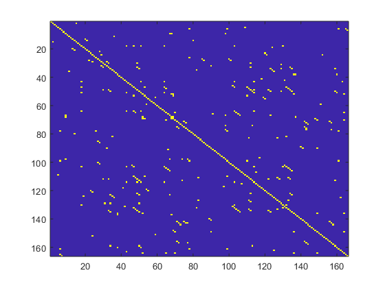
Fig.1 -Typical recurrence plot for a 10-s epoch recorded from retrosplenial area. Note the presence of several lines parallel to the main diagonal line.
The lengths of these parallel to the main diagonal lines describe the duration of which two points in the phase space are close to each other. The embedding dimension and lag were selected to be m = 10 and τ = 1, respectively. The threshold distance r was selected to be √mSD, where SD is the standard deviation of the RR time series.
The recurrence rate (RR) is defined as the ratio of ones and zeros in the RP matrix.
Accordingly, the average diagonal line length (l mean), is obtained as
 where N
l
is the number of length l lines.
where N
l
is the number of length l lines.
In this study, we included only the RQA index lmean. This parameter has been shown to be strongly associated to the largest Lyapunov exponent. (11
For RQA analysis, we slightly modified the Matlab method proposed by Ouyang, downloaded from the site
https://www-mathworks.com/matlabcentral/fileexchange/46765-recurrence-quantification-analysis-rqa.
As result of RQA analysis each 10-s epoch is represented by a vector of 40 lmean values, corresponding to the different brain areas visualized by WFCI.
Association between wake/sleep stage and lmean
For each brain area the linear correlation coefficient was estimated between the lmean value and the numerical value of the sleep score. Assigning a higher value(3) to REM sleep might seem controversial, however, results obtained with this dataset applying multiplex visibility graph (MVG), suggest that this could be a right choice, since REM sleep seems to be associated to larger scale association across the brain. (Fig. 6) 8
Brain Area Scoring
For each area, correlation between area and sleep stage was tested 77 times (11 recordings taken from each of the 7 mice). As significant correlation, a value of R=0.21 was taken (p=0.05). The Brain Area Scoring Index (BASI) is defined as the number of significant correlations counted from all 77 recordings.
Areas were ranked as per BASI values. The three areas showing the highest BASI values were selected.
Association between different areas
To assess the degree of association between two different areas as in a given epoch, the corresponding linear correlation coefficient was estimated. For a given 940-s recording association between two areas corresponding to a given wake/sleep stage, we defined the average of correlation values corresponding to this stage over the whole recording. Since the number of epochs differ for each stage, this index presents certain limitation. At this stage of preliminary analysis, the aim of introducing this index is to have the possibility to carry on nonparametric repeated comparisons. Further studies will require the introduction of a more robust index.
Results
As it can be seen from figure 2, calcium signal time series recorded from the same brain at different epochs (awake and REM) seem to differ both in general appearance and spectral structure.
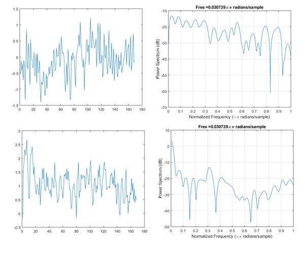
Fig. 2 - Ten seconds time series (left) and corresponding power spectra (right) recorded from the retrosplenial area during awake condition and for REM stage (down).
In figure 3 two representative maps for lmean values obtained from 10-s epochs corresponding to two different conditions are shown. Arrows indicate the area corresponding to retrosplenial area. As obtained in this illustrative example, for this brain area, higher lmean values are exhibited during REM sleep.
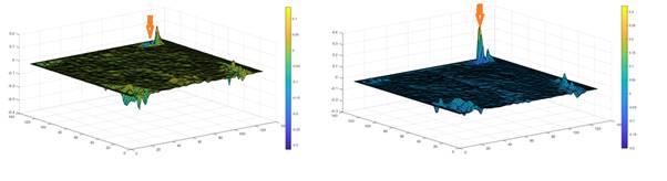
Fig. 3 - Maps corresponding to lmean values for a 10-s epoch with the mouse awake (left) and in REM sleep stage. Arrow indicate values corresponding to retrosplenial area. Corresponding activation with REM is apparent.
Further we analyzed for recording containing 94 10-s epochs the degree of association between the estimated lmean value and the sleep stage, for each of the analyzed areas. In figure 4, the obtained correlations corresponding to different areas are shown for a selected 940-s recording. As noticed, in this case, the strongest association corresponds to the retrosplenial area (indicated by arrow), for which a significant association was obtained (p=0.0000).
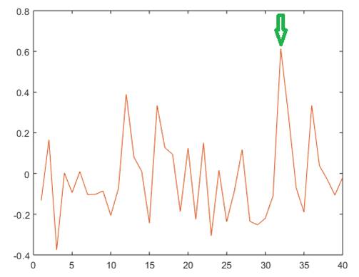
Fig. 4 - Correlation between sleep stage and Imean RQA index for different cortical areas. Notice the high correlation exhibited by Right Retrosplenial Area (marked with arrow).
On the basis of the analysis of all the 77 traces studied, we estimated the BASI scores for each area. We obtained that the highest BASI scores corresponded to retrosplenial, parietal-medial and parietal areas. Surprisingly, these areas are located in a contiguity neighborhood (see figure 5).
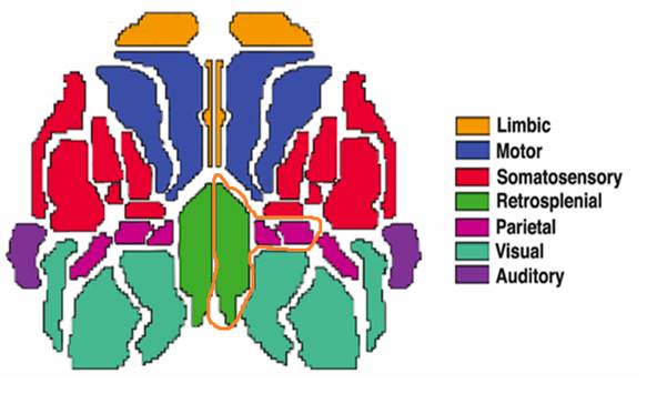
Fig.5 -The three areas with highest BASI scores have been encircled. Note their contiguity in the posterior right area of the brain.
Coupling between areas
We Further decided to explore the degree of coupling between retrosplenial area and medial parietal and parietal areas in relation to the sleep stage. As a criterion of association strength we picked the linear correlation coefficient between signals. We randomly selected ten epochs corresponding to wake state, eleven epochs corresponding to NREM sleep and eight epochs with REM sleep. We observed that the highest correlations were observed between contiguous areas: retrosplenial vs. parietal (0.754±0.103) and parietal vs. parietal medial (0848±0.05). We explored whether the sleep stage influenced the association between areas. We obtained that the association between parietal and parietal medial areas was not influenced by sleep stage, at the same time, the association between retrosplenial area and each of the parietal areas was the weakest in waking state (p<0.05).
Pairwise comparisons
To further explore quantitative changes associated to sleep stage, we averaged the obtained value for lmean for selected areas, as well as the linear correlation for a pair of areas. We analyzed 77 15.66-minutes traces. Results from the 41 traces containing all the three wake/sleep stages were included into pairwise analysis (nonparametric Wilcoxon Matched Pairs Test).
For the right retrosplenial area we obtained that the averaged parameter lmean was higher in sleep_1 stage compared to the wake stage (p<0.05). Meanwhile, no difference was conformed for REM sleep (Table 1).
Table 1 - Pairwise comparison of averaged lmean values as per sleep stage. Nonparametric Wilcoxon Matched Pairs Test. Seven animals were studied. Higher values of lmean were documented for sleep_1 stage as compared the wakefulness.
| Z | ||
|---|---|---|
| Wake & Sleep_1 | 2.313067 | 0.020720 |
| Wake & REM | 0.019438 | 0.984492 |
We also compared the association between right retrosplenial and parietal areas as a function of sleep stage. We obtained that the averaged parameter correlation between both areas was higher in sleep_1 stage compared to the wake stage (p<0.01), as well as in REM sleep compared to wake stage (p<0.01; see Table 2).
Table 2 - Pairwise comparison of mean correlation coefficient between 10-s time series from retrosplenial and parietal areas in relation to sleep stage. Nonparametric Wilcoxon Matched Pairs Test. Seven animals were studied. Higher values of the association between both areas were documented for both sleep_1 stage and REM as compared the wakefulness.
| Z | ||
|---|---|---|
| Wake & Sleep_1 | 3.564623 | 0.000364 |
| Wake & REM | 3.205597 | 0.001348 |
Discussion
We analyzed a publicly available database of WFCI taken from long duration recordings from 7 mice in different wake/sleep stages. As it is known, the frame rate obtained with these traces is much lower than typical sampling rates for brain signals (EEG/MEG). This precludes the investigation of well-established brain frequency-domain features as alpha, beta, and 40Hz activity.
We decided to search for RQA indices given their high performance as biomarkers of different conditions (sleep stages, depth of anesthesia, autistic spectrum), as well as the scale independence of many nonlinear processes from nature, including brain activity.
On one hand, we obtained that the chosen RQA index (lmax) is capable to be associated with the wake/sleep state of the brain. On the other hand, we obtained that the most sensitive areas according to this criterion are located in a relatively small region on the right portion of the brain. This is in accordance with the results obtained by other authors, who found that retrosplenial cortex shows highest accuracy as compared to other regions such as somatosensory and motor cortex. 8
At the same time, we observed that the association between the retrosplenial cortex and parietal and parietal medial increased as the mouse falls asleep. The physiological importance of this association might reveal special interest.
These results motivate for a deeper study of these areas in sleep physiology as well as other important brain functions.
In our opinion, the usefulness of RQA-derived indices for the analysis of WFCI and the association between different areas are promising outcomes from this study. Future directions with this database should include:
A complete sleep classification exercise using the four RQA measures as predictors.
An analysis of interactions between all involved brain areas using RQA-based granger causality analysis, to elucidate network architecture changes associated to different degrees of sleep state.
We expect that such an analysis could serve as a basis for further analysis of WFCI in different situations, including epilepsy, and cognitive performance.
Conclusions
Nonlinear RQA analysis applied to WFCI time series allowed to identify the Retrosplenial and parietal areas as particularly sensitive to changes in sleep waking condition. In particular, our results suggest that the RQA feature lmean decreases in sleep_1 stage compared to waking stage. Sleep (both sta sleep_1 stage and REM) is apparently associated with an increase in the association between retrosplenial and parietal areas. Overall, these results suggest that RQA and association analysis are appropriate to assess modification associated to changes in brain condition, in spite of the poor sampling rate of WFCI signals.

