


 Serviços customizados
 Inglês (pdf)
 Artigo em XML
 Referências do artigo
 Enviar este artigo por email
 Citado por SciELO
  Similares em
SciELO
Similares em
SciELO 
 Permalink
1.-INTRODUCTION
Due to the fast fading effects resulting from multipath propagation, the fields around mobile phone base stations exhibit small scale variations in space. The variation depth (max/min) is typically about 10 dB, but may reach up to 20-30 dB [1]. Therefore human exposure measurements at only one fixed point in space are not representative for the mean or maximum exposure over the volume occupied by the human body.
In [2] the impact of small-scale fading on the estimation of local average power density for radiofrequency exposure assessment was studied in the case of a Rayleigh fading, a Rician-k fading, and a Nakagami-m fading. The authors gave the relation between the error on the estimation of local average power density and the number of independent points that are used in the averaging process. To get some statistical information about fading severity in real environments measurements were performed in a 9-points rectangular grid of 0.5 m x 1.0 m, which matched human body dimensions. At investigated frequencies (>925 MHz), the distance between the sampling points ensured uncorrelated measurements.
Apparently, the results of [2] exerted a great influence on the exposure guidelines and standards for the protection of humans from RF electromagnetic fields that were prescribed or revised after 2005 [3-9]. In the normative documents, the maximum exposure limits for electric and magnetic field strengths and power density are derived from the basic restrictions for the whole-body averaged SAR. When the field distribution along human body is non-uniform these documents recommend performing a spatial averaging process for a whole-body assessment [10]. The field values are then determined at N points (3, 6, 9, 20 or other) as described in [5], [6], [8] and [9]. Three points, at the heights of 1.1 m 1.5 m and 1.7 m above the ground level are basically recommended, except when a higher accuracy is required. The spatial averaging is done on the E 2 or H 2 values, since the exposure limit is based on SAR, which is directly proportional to these values. The concept of spatial averaging of the field strengths is based on the finding that whole-body SAR is related more to the average field strength over the body dimensions than to the peak value at one specific point [11].
Although many spatial averaging schemes have been proposed, no global standard exists regarding number and spatial distribution of sampling points. Thus, according to [5] the local values must be measured over the projected surface (flat plane), equivalent to the head and trunk region of persons (adults or children) who would occupy the area of the incident fields, the measurement points should be uniformly spaced within the sampling area, and the local values should be measured in nine or more points. In [4] the spatial average can be measured by scanning a planar area equivalent to that occupied by a standing adult human, and in most instances a simple vertical, linear scan of the fields over a 2 m height through the center of the projected area will be sufficient. In [6] and [8] the projected surfaces are suitable for an adult human with a height of 1.75 m, and the measurement points (3, 6 or 9) are non-uniformly spaced within the sampling area. In [9] a spatial averaging scan over the vertical extent of an adult human (from 20 cm to 1.8 m) for a temporal uniform electric field is performed, whereas for a temporal non-uniform electric field each point of a uniformly spaced 5-points vertical line representing the vertical extent of an adult human is measured.
In [12] methods were proposed for spatial averaging of the fields emitted by the base stations antennas and for the estimation of the overall uncertainty of the spatial averaged values extrapolated to the maximum traffic configuration. The maximum possible field strengths at every specific point belonging to a spatial averaging scheme were evaluated and the associated uncertainties were estimated. Measurements of the GSM900 and GSM1800 downlink signals were taken in an urban location on a 27-points array in the form of an orthogonal parallelepiped of 0.4 m x 0.6 m x 0.4 m (the reference array) representing the volume of the human body. Thirty-two different combinations of spatial averaging schemes were investigated in relation to the reference array. From the obtained results the tetrahedron-type array with seven points was selected and proposed as the best one.
In [13] the results of an investigation carried out in Korea on the spatial averaging of the fields emitted by the base stations antennas over the volume occupied by human body were presented. The measurements were taken in the vicinity of 6 base stations using a reference 27-points array similar to that used in [12] and three 9 and 6-points rectangular arrays each that were part of the reference one. The results showed that the spatial averages over 9 and 6-points arrays had a mean maximum difference of about 3.1% with relation to the reference value, and that the maximum values appeared with a higher probability in the 9-points array. The author opted for the rectangular 9-points array.
In [14] a spatial averaging method for the magnetic field from the wireless power transfer system of a desktop computer was proposed. Measurements of the magnetic field strength were taken on a 90-points rectangular array of 0.4 m x 1.8 m (the reference array) representing the planar area equivalent to that occupied by a standing adult human. Five different combinations of spatial averaging schemes (rectangular 27 and 18-points arrays, and linear 9, 6 and 3-points arrays) were investigated in relation to the reference array. Taking into account the standard uncertainty of measurements for the obtained differences, the authors selected and proposed the rectangular 18-points array.
It is evident that a tetrahedral volume, a rectangular area or a vertical line segment cannot mimic suitably the projected surface equivalent to that occupied by a standing human body, whose dimensions, moreover, are different for an adult person and for a child, and are located at different distances from the ground. On the other hand, in an appropriate spatial averaging scheme the distance between the sampling points should take into account the small-scale fading correlation distance between two values of the field. Therefore it should vary with the frequency.
In conclusion, the spatial averaging schemes recommended in the exposure guidelines and standards, as well as others proposed in the literature, have deficiencies that prevent the obtaining of more realistic results. The objective of this paper is to present an alternative spatial averaging scheme that can lead to better results.
2.-INVESTIGATION OF THE SPATIAL AVERAGING SCHEMES
A new spatial averaging 18-points scheme (18P) and a 14-point one (14P) were considered and investigated in this work together with other spatial averaging schemes currently in use [5,6,8,9]. These schemes (point arrays) are shown in Figure 1 superimposed to scale to the silhouettes of an adult human (based on the Duke model of the Virtual Family [15]) and of a 6 years-old child (based on the Thelonious model of the Virtual Family [15]). In Figure 2, the distances between the points and the spatial localization of these for the basic configuration of the new investigated 18P and 14P arrays are shown.
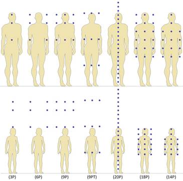
Figure 1 Investigated arrays of points superimposed to the silhouettes of the Duke and Thelonious models.
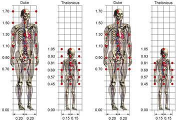
Figure 2 Distances between the points and their localization for the basic configuration of the new investigated arrays.
It can be noticed that the point arrays specified for the spatial averaging of the field strengths in the most used current standards mimic the human figure very poorly. In particular, in the case of an adult person with a height and width similar to those of the Duke model, the 3P, 6P and 9P arrays do not cover an important part of the organs located in the trunk, while although the 9PT array does cover the whole area, in this case the density of points could be too low. On the other hand, the 20P array covers only the region along the axis of the human body. The situation that arises for a child with a height and width similar to those of the Thelonious model is even worse. In fact, in this case the 3P, 6P and 9P arrays cover a region completely outside of that occupied by this model, the 9PT array have three points very far from it, and the 20P array, besides covering only the region along the axis, has almost half of its points outside of the region of interest.
The investigation was based on numerical simulations of the silhouette's models exposure to the electromagnetic fields in the frequency range from 100 MHz to 3 GHz. Six different propagation conditions of a plane wave were considered and the obtained results for the spatial averaging of the electric field strength over the given silhouette were compared with those obtained for the spatial averaging over the points of the given array.
Using the Finite Element Method (FEM) the wave equation for the electric field strength in the frequency domain
 (1)
(1)
was solved in a 2D planar geometry (Figure 3), where ω is the angular frequency, and μ and ε ̃ are the magnetic permeability and the complex permittivity of the medium, respectively: μ=μ
0
μ
r
y 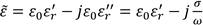 . The solution domain of the problem consisted of three regions: (1)- air, (2)- ground, and (3)- wall. In the exterior boundaries of the ground and wall regions an absorbing boundary condition (no reflection) was applied. In the interior boundaries continuity boundary conditions were used. The exterior boundaries of the air region where treated as a port which was excited with a plane electromagnetic wave having an amplitude E0=1V/m.

Figure 3 Human exposure setup for the investigation of the spatial averaging schemes by numerical simulations. The setup has an incident plane wave, which creates constructive and destructive interference when reflected from the ground and from the wall.
Three values of the incidence angle θ (100o, 120o y 140o) and two sets of values of the relative permittivity εr' and the conductivity σ, selected from [15], where used for the materials of the ground and the wall: (1)- the values of the brick for the wall, and the values of the concrete for the ground, (2)- the values of the refractory brick for the wall, and the values of cellular concrete for the ground. An adaptive mesh of triangular elements with a number of elements between 17402 and 28443 was generated, fixing the maximum element size in 0.2λ, where λ is the wavelength.
Starting from frontal plane bitmap images of the Duke and Thelonious anatomical models, vectorial plane images of these models (the silhouettes) were built to be used in the simulations, where they were considered as part of the air domain. For solving the corresponding linear equation system of the problem the MUMPS code [16,17] was used, with a memory assignation of 1.2 and a pivot threshold of 0.1.
The simulations were performed for 12 values of the frequency: f1=100 MHz, f2=100 MHz, f3=100 MHz, f4=100 MHz, f5=100 MHz, f6=100 MHz, f7=100 MHz, f8=100 MHz, f9=100 MHz, f10=1000 MHz, f11=2000 MHz, y f12=3000 MHz,. The obtained results for the electric field strength spatially averaged over the silhouette of the given anatomical model and over the points of the 7 considered arrays were processed in two different ways, which were referred here as SA1 processing and SA2 processing.
SA1 processing:
First, for the mth anatomical model [m=(1,2)], ith frequency [i=(1,2,…,12)], jth array [j=(1,2,…,7)], and kth propagation condition [k=(1,2,…,6) for Thelonious, and k=(1,2,3) for Duke] the deviations dmijk of the spatially averaged value of the electric field strengths over the considered array, Emijk, relative to the spatially averaged value of the electric field strengths over the silhouette of the given anatomical model, Emik, were calculated:
 (2)
(2)
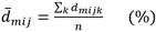
Next, the mean values  of the deviations d
mjk
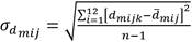
corresponding to all frequencies, and their standard deviations σ
dmjk
were determined:
of the deviations d
mjk
corresponding to all frequencies, and their standard deviations σ
dmjk
were determined:
 (3)
(3)
 (4)
(4)
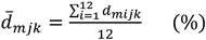
Finally, the relative deviations d mjk of the spatially averaged values of the electric field strengths, corresponding to each given model, array and propagation condition were expressed in the form
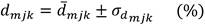 (5)
(5)
In the case of the Thelonious model, this processing was applied to the results of the simulations performed for the 6 different propagation conditions, corresponding to the three considered values of the incidence angle θ and to the two sets of values of the relative permittivity and the conductivity for the ground and the wall. Differently from this, the simulations for the Duke model were performed only for 3 different propagation conditions, corresponding to the three considered values of the θ angle and to the first set of values of the relative permittivity and the conductivity for the ground and the wall. Overall, 12×6×7=504 simulations were performed for the Thelonious model, and 12×3×7=252 for the Duke model. The relative deviations d mjk were visualized using bar plots.
SA2 processing:
First, the relative deviations d
mijk
were calculated as before. Next, the mean values  of the deviations d
mij
corresponding to all propagation conditions, and their standard deviations σ
dmij
were determined:
of the deviations d
mij
corresponding to all propagation conditions, and their standard deviations σ
dmij
were determined:
 (6)
(6)
 (7)
(7)
where n=6 for the Thelonious model and n=3 for the Duke model.
Finally, the 24 vectors of the d mijk deviations, corresponding to each model and frequency for all considered propagation conditions were conformed. For example, the vector d 16jk , corresponding to the 1st model (Duke) and to the 6th frequency (600 MHz) has the form:
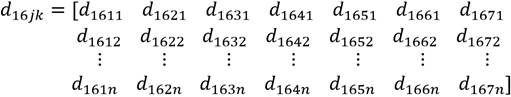 (8)
(8)
The data contained in the previous 24 vectors (12 for the Thelonious model and 12 for the Duke model) were visualized using box plots.
3. - SPATIAL AVERAGING OVER THE DUKE MODEL
In Figure 4 the relative variations of the spatially averaged value of the electric field strengths over the considered arrays relative to the spatially averaged value of the electric field strengths over the silhouette of the Duke model, corresponding to all frequencies (SA1 processing) are shown. It can be noticed that the smallest variations were obtained for the 14P array, although the differences with the 9PT and 18P arrays were small. On the other hand, the variations showed a marked dependence on the propagation conditions: in general a decrease of the variations with the increase of the θ angle was observed, or what is the same, with the decrease of the distance to the source.
In Figure 5 (A, B and C) the box plots for the deviations of the spatially averaged value of the electric field strengths over the considered arrays relative to the spatially averaged value of the electric field strengths over the silhouette of the Duke model, corresponding to the three considered propagation conditions (SA2 processing) are shown. It can be seen that although the means (the green lines) of the deviations for the 14P array showed a tendency to always be among the lowest, they were really the lowest only at the frequencies of 100, 300, 400, 500 and 2000 MHz. At the frequencies of 200, 600, 700, 1000 and 3000 MHz the 9PT array showed the best behavior, while at the frequencies of 800 and 900 MHz the best behavior was shown by the 6P and the 18P arrays, respectively. However, it could be expected that the arrays which have a higher density of points and better mimic the human figure show the best behavior. Of all the examined arrays, the 14P and the 18P are those that better satisfy this condition; nevertheless the better results were obtained with them only in 50% of the cases. It was striking also that with the 6P array, which covers a similar area to that of the 9P, but with a lower density of points, better results were obtained than with this last one in four of the twelve examined cases (frequencies of 600, 700, 800 and 1000 MHz).

Figure 4 Deviations of the spatially averaged value of the electric field strengths over the considered arrays relative to the spatially averaged value of the electric field strengths over the silhouette of the Duke model, corresponding to all frequencies (SA1 processing).

Figure 5A Deviations of the spatially averaged value of the electric field strengths over the considered arrays relative to the spatially averaged value of the electric field strengths over the silhouette of the Duke model, corresponding to the three considered propagation conditions (SA2 processing) for frequencies between 100 and 400 MHz.
Figure 5B Deviations of the spatially averaged value of the electric field strengths over the considered arrays relative to the spatially averaged value of the electric field strengths over the silhouette of the Duke model, corresponding to the three considered propagation conditions (SA2 processing) for frequencies between 500 and 800 MHz.
Figure 5C Deviations of the spatially averaged value of the electric field strengths over the considered arrays relative to the spatially averaged value of the electric field strengths over the silhouette of the Duke model, corresponding to the three considered propagation conditions (SA2 processing) for frequencies between 900 and 3000 MHz.
It should be noticed that none of the examined point arrays covers completely the region occupied by the human silhouette, therefore the result of the spatial averaging of the field strengths over the points of a given array will be so much closer to that obtained over the silhouette, as lesser will differ the spatial distribution of the field strength in the region covered by the array from that existent over the silhouette. The above-mentioned is illustrated in Figure 6, which reveals why at 200 MHz the results of the spatial averaging over the points of 9PT array were better than those obtained over the 14P array, while at 500 MHz the results were the opposite.

Figure 6 9PT and 14P arrays of points and the distribution of the electric field strength over the region occupied by the silhouette of the Duke model for θ=140o and two different frequencies: (a) and (b) - 200 MHz; (c) - 500 MHz.
A deeper analysis of the cases in which the 14P array did not show the best behavior allowed us to notice the important role that should be given to the small-scale fading correlation distance in the selection of the distance between the array points. We proceeded considering the propagation condition that had the major weight on the observed unfavorable result at the given frequency. In the case of 600 MHz this was that of the θ=100o, for which d 1651 resulted to be equal to 17.45% (sub-indexes of d: m=1corresponds to Duke, i=6 corresponds to 600 MHz, j=5 corresponds to the 14P array, and k=1 corresponds to the propagation condition θ=100o with the first set of values for the permittivity and the conductivity assigned to the materials of the ground and the wall in the computational model). In Figure 7 (a) the corresponding results of the simulations of the electric field strength are shown. It may be noticed that almost all the points that form the array coincide accidentally with maximum positions for the electric field strength, which explains why in this case the average value of this magnitude over the mentioned points differs so much from the average value over the silhouette of Duke.
In Figure 7 (b) the results of the same simulations are shown for a new 14P array for which it is impossible that under the given propagation conditions all the points coincide accidentally with positions of extreme values (maximum or minimum). This new 14P array was designed in such a way that the distance d h between the points in the horizontal direction is determined by the small-scale fading correlation distance d c according to
d h =d c ×(n±0.5) (9)
where d c =0.5λ, n=0,1,2,3,… and is selected such that δ=|d h -d h0 | is minimum, being d h0 the distance between the points in the horizontal direction for the basic configuration of the 14P array (0.2 m for the silhouette of the Duke model and 0.15 m for the silhouette of the Thelonious model). It should be noticed that the expression (9) is applicable only when d c is comparable or lesser than the maximum width of the human body. In this work the condition of applicability of (9) was established in the form d c ≤0,7×a, where a is the maximum width of the human body. Accordingly, the expression (9) was applied to the Duke model only for frequencies f≥500 MHz, and to the Thelonious model only for frequencies f≥800 MHz.
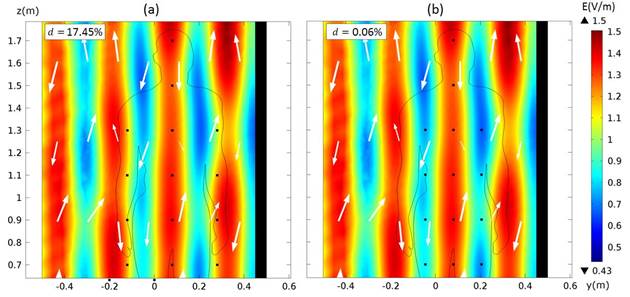
Figure 7 d 1651 deviations of the spatially averaged value of the electric field strength over two different 14P arrays relative to the spatially averaged value of the electric field strengths over the silhouette of the Duke model, corresponding to f = 600 MHz and θ=100o. In (a) the array is the basic one shown in Figure 2, while in (b) the array is the redesigned one considering the small-scale fading correlation distance.
At 600 MHz, d c =25 cm, so using n=0 it is obtained d h =12,5 cm; thus, when the points of the central region of the array coincide with a region of maximum of the field, the points of the periphery coincide with a region of minimum and vice versa. In this case a value of only 0.06% was obtained for d 1651 as it is shown in Figure 7 (b).

Figure 8A Deviations of the spatially averaged value of the electric field strengths over the considered arrays relative to the spatially averaged value of the electric field strengths over the silhouette of the Duke model, corresponding to the three considered propagation conditions (SA2 processing) for frequencies between 500 and 800 MHz. The involved 14P array is the redesigned one (the enhanced) considering the small-scale fading correlation distance.
Although for some values of the frequency and propagation conditions the obtained results of the spatial averaging of the electric field strengths over the points of the new 14P array were lightly worse than those obtained with the basic 14P array, the global result for all propagation conditions at each frequency was always better using the new array. This can be seen from Table 1 where the performance of the basic 14P and the enhanced 14P arrays is compared, and from Figure 8 (A and B) where the deviations of the spatially averaged value of the electric field strengths over the considered arrays relative to the spatially averaged value of the electric field strengths over the silhouette of the Duke model, corresponding to the three considered propagation conditions (SA2 processing) are shown taking into account the small-scale fading correlation distance for the 14P array.
Figure 8B Deviations of the spatially averaged value of the electric field strengths over the considered arrays relative to the spatially averaged value of the electric field strengths over the silhouette of the Duke model, corresponding to the three considered propagation conditions (SA2 processing) for frequencies between 900 and 3000 MHz. The involved 14P array is the redesigned one (the enhanced) considering the small-scale fading correlation distance.
Table 1 Mean values of the d mijk deviations for all propagation conditions, obtained for the spatial averaging of the electric field strengths over the Duke model using the basic 14P and the enhanced 14P arrays
| Array |
|
|||||||
|---|---|---|---|---|---|---|---|---|
| 500 MHz | 600 MHz | 700 MHz | 800 MHz | 900 MHz | 1 GHz | 2 GHz | 3 GHz | |
| 14P basic | 2.43 | 7.26 | 9.89 | 12.14 | 10.06 | 8.39 | 2.54 | 9.07 |
| 14P enhanced | 1.59 | 3.34 | 3.41 | 2.12 | 1.87 | 4.46 | 1.52 | 4.20 |
4. - SPATIAL AVERAGING OVER THE THELONIOUS MODEL
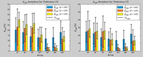
Figure 9 Deviations of the spatially averaged value of the electric field strengths over the considered arrays relative to the spatially averaged value of the electric field strengths over the silhouette of the Thelonious model, corresponding to all frequencies (SA1 processing). (1) and (2) correspond, respectively, to the first and the second sets of values of the relative permittivity and the conductivity for the materials of the ground and the wall.
In Figure 9 the relative deviations d mjk of the spatially averaged value of the electric field strengths over the considered arrays relative to the spatially averaged value of the electric field strengths over the silhouette of the Thelonious model, corresponding to all frequencies (SA1 processing) are shown. As it can be seen, again the smallest variations were obtained for the 14P array; however in this case only the differences with the 18P array were small. As before, the variations showed a marked dependence on the propagation conditions, but in this case a decrease of the variations with the increase of the θ angle was observed only for the 14P and 18P arrays.
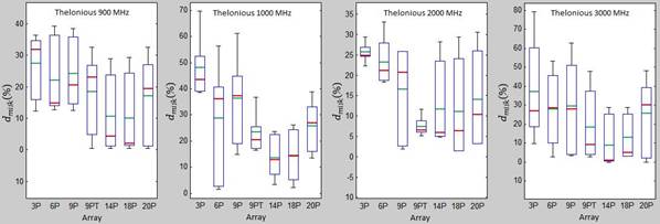
Figure 10A Deviations of the spatially averaged value of the electric field strengths over the considered arrays relative to the spatially averaged value of the electric field strengths over the silhouette of the Thelonious model, corresponding to the six considered propagation conditions (SA2 processing) for frequencies between 100 and 400 MHz.
Figure 10B Deviations of the spatially averaged value of the electric field strengths over the considered arrays relative to the spatially averaged value of the electric field strengths over the silhouette of the Thelonious model, corresponding to the six considered propagation conditions (SA2 processing) for frequencies between 500 and 800 MHz.
Figure 10C Deviations of the spatially averaged value of the electric field strengths over the considered arrays relative to the spatially averaged value of the electric field strengths over the silhouette of the Thelonious model, corresponding to the six considered propagation conditions (SA2 processing) for frequencies between 900 and 3000 MHz.
In Figure 10 (A, B and C) the box plots for the deviations of the spatially averaged value of the electric field strengths over the considered arrays relative to the spatially averaged value of the electric field strengths over the silhouette of the Thelonious model, corresponding to the six considered propagation conditions (SA2 processing) are shown. It can be seen that, contrary to the case of the Duke model, in this case the means (the green lines) of the deviations for the 14P array were the lowest for most of the frequencies, except for the frequency of 2000 MHz, for which the better behavior was shown by the 9PT array, and for the frequencies of 100, 800 and 900 MHz, for which the better behavior was shown by the 18P array, although with little differences with respect to the 14P array. The favorable results obtained for the 14P and 18P arrays must be influenced partly by the smallest spatial dimensions of the Thelonious model in comparison with the Duke model, since in this case the possible differences between the spatial distribution of the field strengths in the region covered by these arrays and the spatial distribution over the silhouette are expected to be lesser. This is well evidenced in exposure scenarios like those shown in Figure 11. Likewise, it is evident that the unfavorable results obtained in general for the arrays different from the 14P and 18P ones must be influenced in great measure by the non-appropriate spatial localization of such arrays in relation to the region occupied by the model under study.
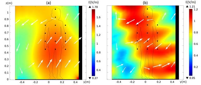
Figure 11 Basic 14P array of points and the distribution of the electric field strength over the region occupied by the silhouette of the Thelonious model for: (a) - f = 200 MHz and θ=120o, (b) - f = 600 MHz and θ=140o. In both cases the first set of values of the relative permittivity and the conductivity for the ground and the wall was used.
As in the case of the Duke model, the results obtained for the 14P array can be enhanced using the correction for the distance between the points given by the expression (9). In Figure 12 the exposure scenario associated to the component d 2951 of the vector d 295k is shown. The effect of the mentioned correction on the computed deviation is evident.
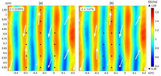
Figure 12 d 2951 deviations of the spatially averaged value of the electric field strength over two different 14P arrays relative to the spatially averaged value of the electric field strengths over the silhouette of the Thelonious model, corresponding to f = 900 MHz and θ=100o. In (a) the array is the basic one shown in Figure 2, while in (b) the array is the redesigned one considering the small-scale fading correlation distance.
Again, for some values of the frequency and propagation conditions the obtained results of the spatial averaging of the electric field strengths over the points of the enhanced 14P array were lightly worse than those obtained with the basic 14P array; however the global result for all propagation conditions at each frequency was always better using the new array. The first statement is illustrated in Table 2 where the six components of the vector d 295k are shown, and the second one is illustrated in Table 3 where the mean values of the d mijk deviations for the six considered propagation conditions, obtained for the spatial averaging of the electric field strengths over the Thelonious model are compared for the basic 14P and the enhanced 14P arrays.
Table 2 Components of the vector d 295k for the basic 14P and the enhanced 14P arrays
| Array |
|
|||||
|---|---|---|---|---|---|---|
| 14P basic | 23.83 | 3.35 | 0.44 | 28.80 | 5.60 | 1.27 |
| 14P enhanced | 1.67 | 2.15 | 3.96 | 1.66 | 2.42 | 5.11 |
Table 3 Mean values of the d mijk deviations for all propagation conditions, obtained for the spatial averaging of the electric field strengths over the Thelonious model using the basic 14P and the enhanced 14P arrays
| Array |
|
||||
|---|---|---|---|---|---|
| 800 MHz | 900 MHz | 1 GHz | 2 GHz | 3 GHz | |
| 14P basic | 11,46 | 10,55 | 13,81 | 12,25 | 9,61 |
| 14P enhanced | 4,08 | 2,83 | 7,14 | 6,05 | 6,49 |
In Figure 13 (A and B) the deviations of the spatially averaged value of the electric field strengths over the considered arrays relative to the spatially averaged value of the electric field strengths over the silhouette of the Thelonious model, corresponding to the six considered propagation conditions (SA2 processing) are shown in box plots taking now into account the small-scale fading correlation distance for the 14P array.
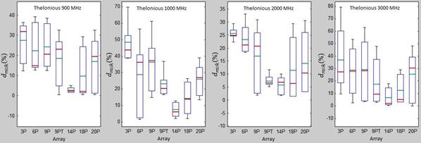
Figure 13A Deviations of the spatially averaged value of the electric field strengths over the considered arrays relative to the spatially averaged value of the electric field strengths over the silhouette of the Thelonious model, corresponding to the six considered propagation conditions (SA2 processing) for frequencies between 500 and 800 MHz. For f=800 MHz the involved 14P array is the redesigned one (the enhanced) considering the small-scale fading correlation distance.
5. - DISCUSSION
From the results obtained for several small-scale fading models in [2] it is evident that when the number of sampling points increases above 20 the uncertainty associated with the estimation of the average exposure over these points relative to the average exposure over the area of the region occupied by them decreases practically little, whereas when the number of sampling points decreases below 12, that uncertainty may increase too fast. Therefore, given that spatial averaging is a time-consuming process, when implementing an appropriate spatial averaging scheme the number of sampling points could be selected not greater than 20 neither lesser than 12 without sacrificing too much the accuracy of the estimation of the average exposure. On the other hand, the implementation of an appropriate spatial averaging scheme should also take into account the dimensions of exposed body relative to the wavelength as well as the figure of the human body. These were the rationales that led us to consider and investigate the 18P and 14P point arrays, and of these two the latter is the proposed one since it yielded the spatially averaged values nearer than those obtained over the silhouettes of the Thelonious and the Duke models. Our results demonstrated also that the 14P array of points can lead to more realistic spatially averaged values, and therefore to more reliable assessments of compliance with safety limits, compared to the spatial averaging schemes recommended in the exposure guidelines and standards, as well as to others proposed in the literature. Although in this work, frontal plane models of the region occupied by the human body were exposed to plane-waves incident from the lateral side, in principle the results must be similar if these models were exposed to plane-waves incident from the frontal side, however in this case the numerical simulations must be performed in a 3D environment.
Figure 13B Deviations of the spatially averaged value of the electric field strengths over the considered arrays relative to the spatially averaged value of the electric field strengths over the silhouette of the Thelonious model, corresponding to the six considered propagation conditions (SA2 processing) for frequencies between 900 and 3000 MHz. The involved 14P array is the redesigned one (the enhanced) considering the small-scale fading correlation distance.
Contrary to the criterion used in [2,12-14] for determining the reference spatially averaged value of the field strengths within the region occupied by the human body, based on point measurements within rectangular areas or tetrahedral volumes, in this work that value is determined by numerical simulations over the region occupied by a planar area equivalent to that occupied by a standing adult human and a child, therefore in this case the investigation of the different spatial averaging schemes under several multipath propagation conditions in connection with their goodness to express correctly the spatially averaged value over that area allows to compare more realistically the performance of these.
6. - CONCLUSIONS AND FUTURE WORK
The results of this work demonstrate that in the frequency range from 100 MHz to 3 GHz the considered 18P and the 14P arrays of points can lead to a more realistic spatial averaging of the field strengths over the human body than other arrays recommended in the exposure guidelines and standards for the protection of humans from RF electromagnetic fields, as well as than others proposed in the literature with the same purpose. Of the 18P and 14P arrays, the last showed the best behavior, and it was further enhanced taking into account the small-scale fading correlation distance between two values of the field.
This work can be helpful for elaborating standards of exposure based on measurements in operating RF systems to assess the real exposure of the human body to these signals. As consequence of the results shown in this investigation, the aspects of the guidelines for assessment of human exposure to RF electromagnetic fields related with the spatial averaging of the field strengths should be modified to include the enhanced 14P array of points as an option.
In a future work the same investigation will be carried out, performing the numerical simulations in a 3D environment.

