


 Serviços customizados
 Espanhol (pdf)
 Artigo em XML
 Referências do artigo
 Enviar este artigo por email
 Citado por SciELO
  Similares em
SciELO
Similares em
SciELO 
 Permalink
Introduction
The main advantage of the Boundary Element Method (BEM) is that it requires discretization only at the limit [1]. Dimension of the input data is smaller and very easy to restructure, which makes it suitable for the problems of moving boundaries, fracture, contact, and stress or fluxes concentration. Due to its mathematical structure, its numerical performance has remarkable accuracy, both in calculating the basic variable and its derivative. Internal values of these variables are still determinate with superior accuracy since the integral boundary equation is reused, and this equation is a new sentence of the weighted residual method [2].
However, a special advantage of BEM consists of the treatment of so-called open or unbounded problems, that is, its domain is infinite or semi-infinite [3]. The discretization of problems of this nature through domain techniques is a difficult challenge because, without an adequate strategy, the traditional approach would generate a large number of equations, making the cost of its solution unfeasible. The BEM, on the other hand, mathematically eliminates the discretization of distant regions. However certain regularity conditions concerning the behavior of the functions in the boundary integral equation on a surface that is infinitely remote from the origin must be fulfilled [4].
Problems with infinite or semi-infinite domains are very important in engineering. Important applications can be mentioned in the analysis of fluid flow profiles in airfoils, in the definition of the thermal profile around fins, in the identification of the cathodic protection potential in submerged pipelines, and many important applications in the area of geotechnics, such as the identification of integrity of the excavated galleries for an underground mine. The Earth, for example, can be considered a semi-infinite medium in determining the temperature variation near its surface. Among many other examples, a thick wall can be modeled as a semi-infinite medium if all that matters is the temperature variation in the region close to one of the surfaces and the other surface is too far away to influence the region of interest during the observation time. Many applications referring to infinite domains can also be related to semi-infinite cases, such as cathodic protection of submerged structures, for example. In addition, considering the example cited, in which the Earth's surface constitutes a case of a semi-infinite medium, there are numerous and important situations where it is desired to make an interface relationship between a solid and a structure and also fluid and a structure. The BEM theory of semi-infinite means applies properly under these conditions, which include geophysics and seismic analysis.
However, it should be noted that there is no abundant material on the theory relating to the application of BEM to these important problems. In the few bibliographic reference [5] the necessary methodological details are not presented, with the exception of the work by Brebbia, Telles and Wrobel [3], which refers to elasticity, theoretical and numerical characteristics related to the BEM approach to problems with open domain have not been reported. This just shows the importance this work has, as there are many peculiarities, especially in treating problems with semi-infinite regions.
Methods
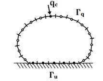
Compared to other numerical methods based on the concept of discretization of the continuum, the Boundary Element Method (BEM) has great advantages; the most important of them is related to require the discretization only in on the boundary, figure 1:
2.1. The Regularity Condition
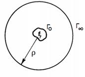
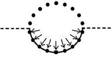
The BEM integral equation for open stationary problems can be obtained by considering a surrounding circle of radius ρ centered on ξ, whose boundary is designated by Γ( and is infinitely distant from the internal boundary Γo, as shown in Fig 2. In this deduction, only an internal boundary was taken; however, the region of interest may contain two or more cavities, whose equation follows the same shown for this simpler situation.
Initially, the integral equation in inverse form involves both the internal and the infinitely distant boundaries, as shown below, equation (1)
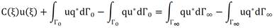 (1)
(1)
In equation (1), u is the primal variable and q is its normal derivative; u * is the fundamental solution and q * its normal derivative.
Equation (1) can be simplified if the source points are located exclusively in the region of interest and the following condition is met:
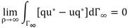 (2)
(2)
This is called the Regularity Condition, which can be obtained in cases where the Saint-Venant Principle [5] is characterized, which states that u and q take the same behavior as the fundamental solution u* and its normal derivative q* in regions sufficiently distant from the point of application of the source or the concentrated thermal loading. Thus, if the loading is applied to an area of interest, at a certain distance from this region, the behavior of the potential reproduces the behavior of the fundamental solution.
In these conditions, for two-dimensional scalar field problems, it can be seen that equation (2) is satisfied, as the two parcels involved cancel each other out when ρ→∞. The Regularity Condition is also obeyed, but in a different way, when the applied request is self-balanced. In this case, it can be seen that the decay of the potential is more accentuated so that the parts of equation (2) cancel each other out separately. A single case of disobedience to the condition of regularity arises when the conditions prescribed in domain Ω are such that they impose uniformity in potential across the whole domain. However, this is not a practical case. Similarly, as infinite domain problems, a semi-infinite problem consists of an idealized domain with a single flat surface that extends to infinity in all directions, as shown in figure 3.
2.2. The Method of Images
Although the theoretical basis is the same, based on the condition of regularity, in the past, the treatment of semi-infinite problems was much less efficient than in infinite cases since significant errors in the solution were introduced by the lack of an adequate fundamental solution. This was only minimized by the use of infinite boundary elements or that had special interpolation. The effective solution to this problem was made with an adjustment in the fundamental solution, made through the Method of Images [6].
The Method of Images (MIM) is a mathematical tool used to solve differential equations in which the domain of the basic variable is extended by adding its reflected image concerning a plane of symmetry. As a result, certain boundary conditions are automatically fulfilled, greatly facilitating the solution of the problem. The MIM is used in electrostatics to calculate the distribution of the electric field of a charge in the vicinity of a conductive surface and can also be used in magnetostatics to calculate the magnetic field of a magnet that is close to a superconducting surface [7]. Its application also occurs in the study of the reflection or absorption of a contaminating plume of a so-called impenetrable outline without flow. Another application of great importance is linked to the study and containment of the propagation of sound outdoors, where acoustic barriers are modeled as bodies without thickness. In this case, their application in the context of the BEM reveals great adequacy and efficiency [8].
In the literature referring to BEM, the Method of Images was initially presented, addressing solutions to the problems of potential [6]. Subsequently, other scalar applications and in cases of elasticity were published [3]. There is a close relationship between the MIM and Green's Functions [9,10] so that the use of the MIM in combination with the BEM can be interpreted as a technique for adapting the classic fundamental solution, so that specific problems related to the semi-infinite regions can be solved. This is because the fundamental solution for the semi-infinite medium can be found by adapting the classic solution for closed media so that the latter automatically satisfies the boundary condition at the interface. In this way, one can dispense with discretizing the semi-plane using the BEM.
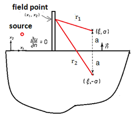
To obtain the fundamental solution adapted from the idea of the MIM, it is necessary to consider the mathematical steps that follow, which also list physical considerations about the problem. Initially consider a two-dimensional space, figure 4, where is applied a source m with coordinates (ξ; a). It seeks to understand what happens at another point located symmetrically to x1 axis that is defined by the interface. This point, called the image source, is positioned exactly at a distance 2a from the original source.
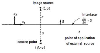
If the reflection condition at x2 = 0 is imposed, the mu* potential field produced by the source m applied in point (ξ; a) will be accompanied by a similar effect produced by the source image m' located in the reflected region. Naturally, the value of m' depends on the type of boundary condition imposed on the interface. The condition of reflection or physical symmetry of the potential is of the greatest interest, as this is much more useful for the practical applications of BEM. As the interface is defined along the x-axis and the direction of normal is in the same direction as y, this implies that, as a reflection boundary condition, one has, equation (3):
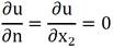 (3)
(3)
Thus, the fundamental solution of the semi-plane results, equation (4):
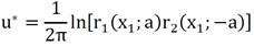 (4)
(4)
With the fundamental solution, it is necessary to derive it to obtain the potential derivative, hereinafter named as the fundamental flux. It is noticed that this is a simple operation, from which it follows equation (5):
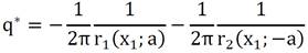 (5)
(5)
It should be noted that in equation (5) the values of r1 and r2 have their well-defined meaning. They are distances from the source and image source points to the field points. In cases where the interface is straight and there are no external sources, these expressions of the fundamental flux cancel each other out at the interface if the field points are located along with it, as shown in figure 5. It is noticed that, in this condition, the distances r1 and r2 are equal; but, because the points are situated symmetrically to the semi-plane, the expressions of q*, although they disappear, end up canceling each other due to the opposite sign of the normal being different in each case. Such a situation occurs in most applications in problems of electromagnetism, an area in which MIM is widely used.
 Source:authors
Fig. 5 Field point located on the interface and symmetric sources located inside the semi plane.
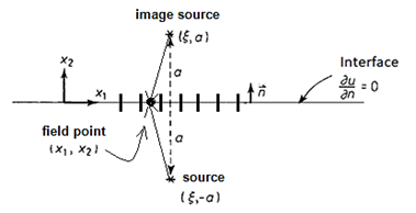
The value of q* is also canceled if the source and field points are both on the interface, as shown in figure 6 below:
Thus, the image source point and original source point have the same position; in this condition, the value of fundamental functions degenerate to the usual Green’s BEM function; however, the MIM fundamental solution needs to be used to guarantee the suitability of the symmetry of semi plane model and eliminating the discretization of the boundary parts with prescribed Dirichlet condition.
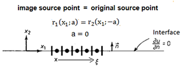
A different situation occurs if there is any irregularity in the semi-plane, figure 7, as in this case r1 is different from r2 and, consequently, q* does not cancel out in the curved boundary:
The most common case in acoustics is when there is a sound source, the effects of which must be attenuated to avoid resonance and produce acoustic comfort. In this situation, figure 8, it is also necessary to introduce a concentrated source, a component that is relatively simple to introduce with the BEM.
 Source:authors
Fig. 8 Usual configuration concerning acoustic source problem: field point and source point located out of the interface.
2.3. BEM Integral equation for semi-infinite media
The integral equation of the BEM studied for the infinite medium remains in the essence for the mathematical model of semi-infinite cases, including the conditions of regularity, which are fulfilled. In other words, the fundamental solution to semi-space also guarantees that the behavior of infinitely distant variables can be neglected due to the decay of u* and q*. However, there are important aspects when obtaining the fundamental solution modified by the MIM.
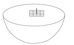
First, consider the semi-infinite medium, as shown in figure 9. In many cases, the region of interest is not the surface defined by the semi-plane but an internal region Γ´, as in the analysis of excavated galleries in a shallow depth mine.
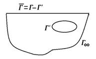
Then, both the boundary interface and the internal boundaries can be loaded. The integral equation of the BEM in this case is equation (6):
 (6)
(6)
Because q* is null in the flat interface, equation (7):
 (7)
(7)
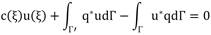
Thus, therefore, any Dirichlet conditions are not applicable in the interface, as previously highlighted. However, the most important aspect is that only the parts of the semi-plane boundary that are submitted to non-zero flux conditions need to be discretized since the fundamental solution is in charge of eliminating them from the model. The singularity in the arguments of the fundamental solution and its normal derivative in the event of a coincidence between the source and field points are also resolved in the same way as in the classical BEM for closed media since u* is a logarithmic singularity, which can be integrated in the usual sense. It is an improper integral, but as it has a weak singularity, it is integrable. The singularity in q * does not exist since the fundamental solution itself was generated based on the annulment of its derivative in the interface. Thus, the standard procedure of the BEM applies to these problems, that is, after the discretization, a classical matrix form is generated in case the field points are located in a curved part of the interface, equation (8):
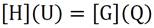 (8)
(8)
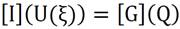
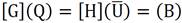
In equation (8), U and Q are potential and flow line matrices, containing known nodal values as well as values to be calculated. G and H are matrices from the weighting integrals for the potential and potential derivative, respectively [1]. The same happens if there are field and load points in any internal boundary, close to the interface. In this case, the number of source points must also be equal to the number of field points, as required usually with BEM.
In the case of applications with straight boundaries and loads only applied to this, aiming at the determination of potentials or fluxes outside the interface, the integrals containing q* cancel each other out - the matrix H disappears - and the system remains only in the equation (9):
 (9)
(9)
In equation (9), I is the identity matrix. In this case, the coefficient c(ξ) that occurs on the diagonal of matrix H [3] is automatically determined by the fundamental solution, which would apparently degenerate to twice the value concerning the classical fundamental solution. However, this does not happen: one source point is inside (c(ξ) = 1) and the other outside the region (c(ξ) = 0) and equivalence with the usual value c(ξ) = 0,5 is obtained.
It is noteworthy that obtaining potential values at the interface happens without the need to solve any system of equations, which is a huge computational advantage. Obviously, the same goes for calculating the values of the potential or flow, if desired, at points located within the semi-infinite domain.
Results and Discussion
3.1. Load concentrated on a straight surface
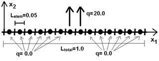
In this first example, a constant flux is applied in a very small part of a straight interface, as shown in figure 10. It is emphasized that the boundary elements are constant and thus the applied load does not extend to neighboring elements, whose condition prescribed is flux null. The interest here is to reproduce the fundamental problem. It is possible to further reduce the interval, considering only one element, but from the presented way it will already be possible to see that the solution of this case in internal points is close to the behavior given by the fundamental solution, adjusted to a flow value that is not unitary, it is equal to 20.
The temperature or the potential results in the boundary are shown in table 1. If the flux (or normal derivative of potential) were effectively singular, the value of temperature would be infinite. Initially, the strategy used here to assess the consistency of these results on the boundary is to calculate numerically the potential values at internal points - whose methodology is based on the Method of Images - and at some points slightly distant from the boundary, but which are equidistant from these. To better illustrate the exposed procedure, figure 11 shows a potential evenly distributed in a semicircle.
Table 1 Temperature on the boundary, example 1. Source:authors
| x1 | x2 | Potential |
|---|---|---|
| 0,025000 | 0,000000 | -0,475105 |
| 0,075000 | 0,000000 | -0,546209 |
| 0,125000 | 0,000000 | -0,626312 |
| 0,175000 | 0,000000 | -0,718046 |
| 0,225000 | 0,000000 | -0,825409 |
| 0,275000 | 0,000000 | -0,954936 |
| 0,325000 | 0,000000 | -1,118491 |
| 0,375000 | 0,000000 | -1,341674 |
| 0,425000 | 0,000000 | -1,704284 |
| 0,475000 | 0,000000 | -2,443571 |
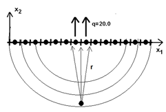
Table 2 presents the results of this comparison between values calculated internally and on the boundary. It can be seen that there is a very satisfactory agreement in the results. The greater error was observed only in the potential value referring to the last node, from which the discretization was truncated. It should also be considered that the values obtained internally are calculated through the reuse of the integral equation, which results in numerical values of greater precision compared to the values calculated on the boundary nodes [2,11].
Table 2 Potential in equidistant points. Source:authors
| x1 | x2 | Internal Potential | Boundary Potential |
|---|---|---|---|
| 0.500 | -0.175 | -1.101152 | -1.118491 |
| 0.500 | -0.375 | -0.622539 | -0.626312 |
| 0.500 | -0.500 | -0.440214 | -0.475105 |
Table 3 compares the analytical values, based on the behavior of the fundamental solution and numerical values at internal points along the line x1 = 0,5. At these points, the so-called analytical values were calculated considering that, from a reasonable distance from the free surface, the vector radius r varies little, since the loaded sector is very restricted and integration errors are not very important. It is observed that, despite the restrictions mentioned for such a comparison, there is a very good agreement between the analytical and numerical results.
Table 3 Analytical and numerical values of potential in internal points. Source:authors
| x1 | x2 | Internal potential | Analytical potential |
|---|---|---|---|
| 0.50 | -0.50 | -0.440214 | -0.441270 |
| 0.50 | -1.00 | 0.000265 | 0.000000 |
| 0.50 | -2.00 | 0.441338 | 0.441270 |
| 0.50 | -5.00 | 1.024611 | 1.024600 |
3.2. Potential uniformly distributed in a semicircle
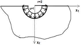
Numerically, this example is quite different from the previous one, since boundary conditions involving both potential and flow can be applied, because they are prescribed in a boundary that does not belong to the interface. Figure 12 illustrates the proposed problem: this is the case where a uniform and unitary temperature potential is applied along the semicircle with a radius equal to two.
When there are no fluxes applied to the interface and the region of interest is symmetrical, this problem is equivalent to the bottom (or top) of a problem with an infinite domain. In this case, there is a simple solution for comparison, which is based on the behavior of the fundamental solution.
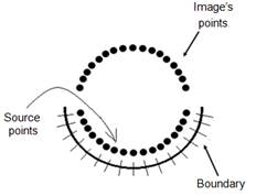
As mentioned, discretization is limited to the semicircular boundary. In this case, unlike the previous cases, both matrices H and G are generated. Figure 13 illustrates the discrete model adopted, in which image source points are positioned symmetrically to the usual BEM source points.
 Source:authors
Fig. 13 Semicircle discretization with field points and source points on the boundary.
The BEM matrix system to be solved equation 10:
 (10)
(10)
Thus, only flows are calculated on the boundary. It is noteworthy that the fundamental solution and its normal derivative, referring to the semi-plane, must be used in this case and in similar problems. Such fundamental solutions allow that it is not necessary to make any discretization along the interface, since the condition of symmetry is naturally incorporated into the problem.
The analytical solution of the problem in an infinite medium with radius r = 2 and the use of the classic fundamental solution indicates a flux value on the boundary equal to 0,72135. The discrete model used here, with 20 constant boundary elements, resulted in an average value equal to 0,713453, with a relative percentage error of approximately 1 %. Although very close, these numerical values can certainly be reduced by refining the mesh, thus eliminating errors in the representation of circular geometry and problems in the corners.
For the internal points, the numerical values obtained at remote points are also satisfactory and are shown in table 4 below, accompanied by the analytical values. It is noteworthy, once again, that the results inside are more accurate than the boundary values. In numerical terms, it should be noted that due to the original source points being on the boundary, the diagonal coefficients of the matrix H referring to the integration based on these points is equal to 0.5, as the elements are constant. The coefficients generated by the image source points have c(ξ) equal to zero, as these points are physically in a void.
In cases where the problem has a vertical symmetry, it can be seen that the H coefficients are practically null, when obtaining the values at points located on this vertical axis of symmetry.
Table 4 Numerical values obtained at points away from the boundary. Source:authors
| x1 | x2 | Potential (BEM) | Potential (analytical) |
|---|---|---|---|
| 0,00 | -3,00 | 1,567359 | 1,583460 |
| 0,00 | -4,00 | 1,977610 | 1,997700 |
| 0,00 | -5,00 | 2,295847 | 2,319110 |
| 0,00 | -6,00 | 2,555877 | 2,582550 |
Still, in the context of this same example, a new arrangement of the source points is presented. Unlike what was done before, the original source points were placed at a distance from the central nodes, this distance is equivalent to the size of the element (0,5), where it was strategically selected so as not to produce appreciable errors of integration, see figure 14. In this condition, the coefficient c (ξ) is equal to zero.
The numerical results were around 0,7242. Compared to previous results with the original source points coinciding with the nodal points, the results had slightly higher precision.
Conclusions
Two typical problems were solved, in which the features of the BEM approach in semi-infinite were clearly presented. Despite the use of constant elements and not very refined meshes, numerical results obtained showed satisfactory accuracy, confirming that the BEM is the most adequate technique even today to solve such problems.
The reference solutions were taken based on the behavior of the fundamental solution in infinite media. For more complex problems, especially when the domain geometry is irregular, it is difficult to find an affordable and reliable reference solution. However, in view of the good results obtained in the tests shown, it is expected that the method has satisfactory precision to solve these more challenging cases.

