


 Serviços customizados
 texto em
  Inglês (pdf)
 Artigo em XML
 Referências do artigo
 Enviar este artigo por email
 Citado por SciELO
  Similares em
SciELO
Similares em
SciELO 
 Permalink
INTRODUCTION
Carrying out the appropriate conservation in the post-harvest stage of the products is among the main steps aimed at achieving food sovereignty and improving the efficiency in the use of agricultural products, which is only possible if a quality product is available with a high degree of acceptance (Hernández et al., 2005; García, et al., 2010; Mogollón et al., 2011; Fernández et al., 2012; Ramos et al., 2013; Jímenez, 2015; López, 2017).The quality of agricultural products refers to a series of attributes fundamentally related to their general health and commercial life. The knowledge of their main physical-mechanical and organoleptic properties using traditional methods and, more recently, the non-destructive ones, plays an indispensable role for a good presentation and conservation of them, which allows defining the most appropriate management during the periods of pre-harvest, harvest and post-harvest (Schofield y Wroth, 1968; Yirat Becerra et al., 2009; Mogollón et al., 2011; Jiménez, 2015; López, 2017). The non-destructive methods have the possibility of being used for the automation of online selection processes and in the development of scientific research since it is possible to homogenize the criterion of selection of samples for studies where several qualities of the fruit intervene and that, historically, were carried out using the criteria of experts. (FAO, 2018). In recent years, as a result of the development of electronics and computers, considerable progress has been made in the use of these applications for teaching and research purposes. That is demonstrated in the proposal in which studies of quality applied to fruits are repeated from new forms and methods derived from the technological development, such as those related to modeling and simulation of fruits or processes that occur essentially during the post-harvest stage. It facilitates making measurements less cumbersome and more precise, also enabling the non-destructive monitoring of this important attribute for fresh fruits, during storage at room temperature (Park,B., et..al., 2001., Garcia ,2007).
On the other hand, the use of Finite Element Method (FEM) for the simulation of mechanical response to static charges (Silvestre, 1998., Lu et al, 2006., Jamal et al, 2005., Kabas, et al, 2008), that is a tool for performing non-destructive tests on fruits, allows predicting optimum storage and handling conditions during transportation in order to improve harvest and post-harvest processes to maintain their quality. During last three decades, the method has been successfully applied in Cuba in the field of agricultural engineering, fundamentally in modeling soil-agricultural implement interaction (Herrera et al., 2008; Martínez et al., 2011; López, 2017). The study aims to characterize from the use of mathematical tools, the post-harvest behavior of the main physical, chemical and mechanical properties linked to the quality of agricultural products.
MATERIALS AND METHODS
Through the Mexican Standard (NMX-FF-041-SCFI-2002) the selection of guava fruits (red dwarf) and pineapple (cayena lisa.) was carried out. A total of 110 fruits was sampled (40 guavas and 70 pineapples), 10 fruits were removed daily, during the experimental days and, for guava, they were divided into two groups by states of maturation (only two states being chosen because the fruit is usually collected for export in state I, that is green) and is usually more susceptible to damage in state III (mature). Due to that they are the most interesting and consist of 20 fruits each. Those 20 fruits of each state are divided into groups of 10, one group to determine mass, density and firmness at compression to 3% of the polar diameter (Ф), and a group of 10 for the determination of the elasticity limit, Young's modulus and Poisson's coefficient.
The size is obtained by polar and equatorial diameter with the use of a caliper from 0 to 150 mm ± 0.05 mm. The mass is determined with an electronic balance model LG-1001ª / 0.1 (g), making three repetitions per fruit and determining the weight losses by Equation 1. The IC was determined by the method of capturing images, photographing the fruits with a digital camera model CANON PowerShot A630 8.5 mega-pixels, then exported to the portable software ADOBE PHOTOSHOP v.10, obtaining the numerical representation of the variables L * a * and b *, which establishes coordinates in a color plane that creates the maturation scale by its coordinates (García et al., 2010).
 (1)
(1)
The contents of soluble solids (SSC, for its acronym in English) are evaluated and density is determined through the principle of Archimedes.
Resistance to penetration (firmness): It was obtained from the puncture test for the case of pineapple and compression to 3% of the polar diameter in the case of the guava, with the digital durometer, Model CEMA-C08, 0 to 1000 (kgf / cm2) / 0.01 (kgf / cm2), of national manufacturing, according to the Magness-Taylor principle in three equidistant points, separated at approximately 120º of others (for whole fruits), according to Hernández (2005). This test was carried out without removing the skin from the fruits.
In the case of guava, two maturation stages were evaluated on the first and third day of harvest, determining firmness at compression (N), 3% polar diameter (10 fruits per ripening stage), the contact area, (mm) and deformations of the polar and equatorial diameters, (mm) to obtain the modulus of elasticity, Poisson's coefficient and the elastic limit, according to González et al. (2015 and 2016).
Limit of elasticity: It was determined by using methodology proposed by Silling (2000), using a force meter (durometer model CEMA - C08 with a flat strut), a vernier caliper and a video camera. The average efforts of the fruits are determined through MATH CAD PRO 2000 program (Essential Mathcad for Engineering, Science, and Math (2000), which is based on the Equation 2.
Young's Modulus or Apparent Elasticity Coefficient: It is determined according to Equation 3. The contact area is determined by marking the durometer plate with chalk powder, so, the area touching the fruit will be marked on it and subsequently obtained using a vernier caliper.
 (3)
(3)
Where:
E |
- Modulus of elasticity |
F |
- Maximum firmness to compression before breaking the fruit |
L1 |
- Longitudinal diameter |
A |
- Contact area |
L2 |
- Deformation of the longitudinal diameter. Apparent Poisson Coefficient (μ) are quantified from Equation 4, and with the help of a caliper (Sharma et al., 2003; Ciro et al., 2005). |
Since ΔD is the transverse deformation, Do the initial transverse length; with ΔL as longitudinal deformation and the initial longitudinal dimension, expressed in mm.
 (4)
(4)
Where:
ΔD |
- transverse deformation |
Do |
- initial transverse length, mm |
ΔL |
- longitudinal deformation |
Lo |
- initial longitudinal dimension, mm |
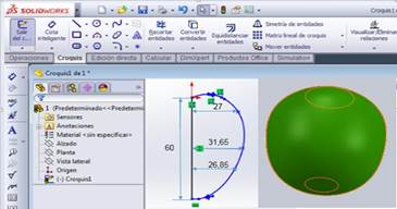
The simulation of static charges in a homogeneous body was made with the help of SolidWorks 2013 program. For the construction of the initial sketch (guava fruit), establishing average measurements (length and equatorial diameter), (Figure 1) in order to establish the appropriate geometry of the material. Once the solid is created, the program is fed with the physical and mechanical properties that characterize the fruit (density, Young's modulus, elasticity limit and Poisson's coefficient). Subsequently the analysis is performed by the Finite Element Method using two models, one for each state of maturation in terms of the deformations determined with the area of the plate-metal fruit and another one with the integrated area, in order to compare the simulated and experimental longitudinal deformations.
To evaluate the error of the model (EM) Equation 5 was used.
 (5)
(5)
RESULTS AND DISCUSSION
Pineapple Properties: Table 1 shows the average values obtained in each of the main properties of quality evaluated in the case of pineapple, note that in this variety (Cayenne Lisa) the mass reached a maximum value of 927 g and a pH of 4.56.
TABLE 1 Average values obtained in the main pineapple quality properties.
| Properties of the Pineapple | ||||||
|---|---|---|---|---|---|---|
| Mass, g | Size, mm | Firmness, kgf/cm2 | IC* | SSC, 0Brix | pH | PP, g |
| 927 | 160 | 4.36 | -0,28 | 14.01 | 4.56 | 14,94 |
Results of Processing the Information Referred to Pineapple Quality
At the end of the evaluated period (Figure 2) weight losses (PP) are very significant, being those corresponding to the start and the second day of measurements, different from the eighth and tenth days (99% confidence level). As it can be seen, weight losses of intermediate days do not differ significantly from one or the other group of means. In the case of firmness, there is a decreasing trend with the days of storage. This is due to several changes that naturally accompany maturity in most fruits, among them the changes in texture and reduction of firmness. With senescence, phenomena such as the degradation of the walls, enzymatic activation, the increase in membrane permeability, among others, cause a decrease in the firmness of the walls of the fruit. The principal component analysis procedure then extracts or proposes five components, from which the first two components were chosen. The choice takes into account those self-values greater than or equal to 1.0 or, what is equal, the components that manage to explain more than 10% of the variance. These first and second CP explain 88% of the variability in the original data, which, as a whole, indirectly characterize the pineapple quality standards during post-harvest storage at room temperature. This result reaffirms that not only the well-known firmness, but weight loss, pH, IC and SSC are suitable indicators to qualify the quality of the fruit and also confirms its use for these purposes as a trend in the literature.
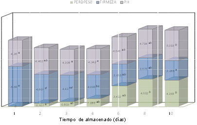
FIGURE 2 Multiple comparisons test applied to the properties to discern the groups of means that differ significantly during the storage time. Different letters indicate significant intergroup differences for p <0.01.
Figure 3 shows the conglomeration or grouping of variables practiced to weight loss, firmness, IC, pH and SSC with three well-defined resulting groupings, which are framed in specific days of storage of the fruit after harvest.
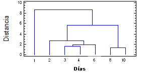
FIGURE 3 Cluster dendogram of weight loss, firmness, IC, pH and SSC generated considering the nearest neighbor method and the Euclidean distance squared.
The pattern of temporal quality variability of pineapple represented by these groupings properties is a valuable tool that excludes the need of carrying out an exhaustive control of these properties during its commercialization, transport or storage and even supplying the lack of instrumentation for their determination. This largely makes it a non-destructive tool to monitor the quality of the fruit in storage.
On the other hand, Figure 4 shows the models adjusted to the different tendencies or temporary variations of weight loss, firmness, SSC and pH, where both measured values are plotted during the ten days of storage and predicted by the models at half-day time intervals. In the case of the predicted values, these are extrapolated a few days later, which took into account not too far from the period of interest, as well as the temporal brevity of the process being analyzed. All the trends described by the models after ten days of storage are considered adequate and are result of the irreversible physiological changes that occur in the fruit, as can be seen with the rise in pH that is subject to the continuity of the fruit maturation.
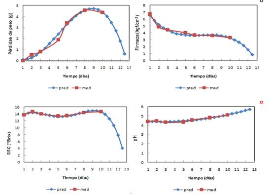
Table 2 shows the adjusted functional dependencies and the statistics that evaluate the adjustment of the model, reaching values of statistics as R2 statistic that indicates that the adjusted model is able to explain up to 99% of the temporal variability of weight losses. This model presents a standard error of the estimate of 0.23, which is why it is considered favorable to accurately describe the pineapple storage process at room temperature.
TABLE 2 Models adjusted to the values of each property and the statistics of its evaluation.
| Property | Model | R2 | MAE | |
|---|---|---|---|---|
| PP | Y = 0,12-0,07*t+0,24*t2-0,02*t3 | 0,99 | 0,11 | 0,23 |
| Firmness | Y = 6,52-1,58*t +0,28*t2-0,02*t3 | 0,98 | 0,13 | 0,24 |
| SSC | Y = 13,79+1,25*t -0,83*t2+0,16*t3-0,01*t4 | 0,89 | 0,14 | 0,30 |
| pH | Y = 4,40-0,04*t +0,02*t2 | 0,97 | 0,04 | 0,06 |
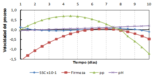
On the other hand, there is no tendency to represent the residues, which means that the variables taken into account are well represented in the model, as pointed out by Donatelli et al. (2004) and Borgesen and Schaap (2004) in the development of pedotransference functions to estimate the soil moisture retention curve. The speed with which the changes in each property measured during pineapple storage occur, can be seen in Figure 5. That graph shows the general dynamics of the processes that take place during the fruit storage at room temperature, particularized through the set of properties evaluated, which are closely related to pineapple maturation and quality (Var. Cayena Lisa). As it can be seen, the maximum speed of weight loss is reached between the fourth and fifth day of harvesting and stored at room temperature (0.7 g / day) and from sixth to seventh day the maximum for the firmness ( 0.04 kgf / cm2day). While the speed and average change rate during the entire storage period of these are 0.17 g / day and -0.04 kgf / cm2 day, respectively. In addition, the greatest degradations of the pineapple, in terms of quality, take place between the fourth and seventh day. The behavior of these properties (SSC and pH) are very contrasting to the previous ones (0.08 ° Brix and 0.08, respectively). Nevertheless, these extremes of the process, it is a gradual and cumulative phenomenon, so it should not be ignored or downplay the overall result.
Similar analyses to those of pineapple are made for the physical-mechanical properties of guava by states of maturation (Table 3). It also shows average diameters that make up the size of the fruit during the analysis and its classification according to size, as in the norm consulted NTC-1263: 2007, as well as the average values of mass and density.
TABLE 3 Average values of the main physical-mechanical properties of guava by states of
| D polar, mm | D equatorial, mm | Mass, g | Classification | Den, g/cm3 | |
|---|---|---|---|---|---|
| EM-I | 60.24 | 60.34 | 119.53 | Grande | 1.01 |
| EM-III | 63.24 | 61.3 | 152.48 | Grande | 0.96 |
The changes of the firmness of guava, expressed as compression force (Table 4), is illustrative of those that occur in the ME that fruit transits through, coinciding with Hernández et al. (2005). As a whole, values reached of its elastic limit (point A), biocedencia point (point B), point of fracture (point C) and compression of the fruits up to 3% of its polar diameter are shown, and there is a significant difference between the MS.
TABLE 4 Average firmness of the fruits for each stage of maturation.
| Firmness (N) | EM-I** | EM-III** |
|---|---|---|
| Force at 3% (A) | 58,0 | 10,4 |
| Force (point A), | 531,5 | 49,0 |
| Force (point B), | 600,5 | 67,1 |
| Force (point C), | 804,8 | 81,9 |
The stress-unitary deformation curves for each MS (Figure 6) for the fruit-metal plate area and the integrated area are plotted and its elastic limit is defined. From these curves the values of the elastic limit (A) are riched and the Young's Module by areas and EM. Table 5 shows their averages along with those of the Poisson coefficient obtained for each ME, which are used to characterize the material, and simulate the firmness of the fruits during the post-harvest stage in the SolidWorks 2013.
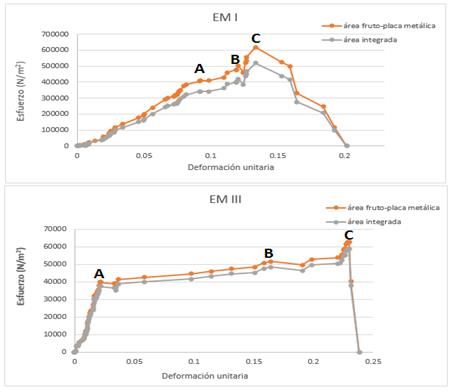
According to the results obtained, it can be observed that as the fruits reach the EMIII, μ decreases because the material resistance decreases with the maturation, being more easily deformable for minor efforts. The values of the modulus of elasticity in the EM-I for the area fruit-metal plate and integrated area show remarkable changes of 4.44 to 3.71 MPa, not happening in the EM-III where the value for the fruit area - metal plate is 1.84 MPa and for the integrated area is 1.78 MPa.
Simulation of Static Charges in a Homogeneous Body
The generation of a mesh small enough to obtain reliable results is one of the most important steps in the simulation, since it must be able to solve the problem under study with a high precision and depends on a convergence analysis. The total number of nodes in this case was 10433 and the total number of elements 7045 (Figure 7).
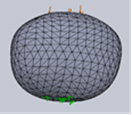
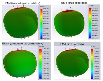
Figure 8 shows changes in the longitudinal deformations (mm), in the z direction, as the fruit moves from EMI to EM III. The fruit, in state of maturity one (EM-I), which is simulated with the modulus of elasticity that takes into account the fruit-metal plate area shows values of longitudinal deformation of 0.94 mm and the one that was simulated with the modulus of elasticity, assuming the integrated area of the fruit, reaches values of 1.12 mm, obtaining a simulation with the latter more approximate than the one obtained experimentally where values of 1.13 mm were recorded for a force of 58 N.
In the case of the state of maturation three (EM-III), for a load of 10.4 N, values of longitudinal deformation of 0.44 and 0.48 mm are obtained in fruits with fruit area-metal plate and integrated area, respectively. These values are closer to those obtained experimentally. In the opposite direction (equatorial diameter), the deformations are small, in the order of 1 to 2 mm, which does not represent a value to be taken into account with respect to those obtained in the contact zone between the fruits and the metal plates.
Comparison of the Results of the Experiment and the Numerical Analysis
Table 6 shows the comparison of both results (numerical analysis using the MEF and laboratory experiment), regarding the longitudinal deformations (ΔL) that occur with the application of compression loads for 3% of the polar diameter.
TABLE 6 Comparison of the average deformations obtained.
| EM | Fmax, N | DL, mm | |
|---|---|---|---|
| Exp. | M E F | ||
| EM-I (fruit -metal plate area) | 58,0 | 1,15 | 0,94 |
| EM-I (integrated area) | 58,0 | 1,12 | |
| EM-III (fruit area-metal plate) | 10,4 | 0,49 | 0,44 |
| EM-III (integrated area) | 10.4 | 0,48 | |
To validate the model, it is necessary to determine the prediction errors of the model, in each of the analyzed variables, where the experimentally obtained values are compared with those derived from the evaluation of the digital model. It can be observed that, in all the states of maturation, a precision of the model greater than 80% is obtained, and in those corresponding to the model (integrated area), it is greater than 90%, table 7.
CONCLUSIONS
With the use of mathematical and simulation techniques, the behavior of properties in pineapple are described and the maximum effort that guava fruit resists in two stages of maturation under static loads, is predicted.
The quality pattern of Cayenne pineapple, stored at room temperature, quantified from weight loss, firmness, pH, contents of soluble solids and color index, is distinguished by three periods corresponding to initial day, between two and six days and between seven and ten days of fruit storage.
The average speed or rate of change of pineapple weight and firmness losses are 0.17 g / day and -0.04 kgf / cm2 / day, respectively, during the entire ten-day storage period at room temperature, while that of the pH and contents of soluble solids is, in both cases, of only 0.08 units per day.
Guava as fresh fruit has average values of height, density and Poisson's coefficient of 60 ± 5 mm, 0.98 g / cm3, 0.41, respectively.
In the module of fruit elasticity in EM-I (fruit -metallic plate area and integrated area) remarkable changes of 4.44 to 3.71 MPa are shown, which do not happen in EM-III, where the values for the fruit-metal plate area is 1.84 MPa and the integrated area is 1.78 MPa.

