Original Article

Spatial-Temporal Characterization of Coverage with the Use of Geoinformation in Miranda Municipality

MSc. Lexa Dayana Pineda-Santos^{I  *}  , MSc. Jorge Eduardo Suárez-Hernández^I 

^IULA-NURR, Villa Universitaria, La Concepción de Trujillo, Municipio Pampanito, Estado Trujillo, Venezuela.

ABSTRACT

The municipality of Miranda, in Trujillo State, is crossed by Pan-American Highway, which is the most important road in the lower area of the state. Its agricultural areas are watered by El Cenizo irrigation system and by other natural channels. The main agricultural activity is sugarcane crop. A characterization of the contamination was made from information taken in the field (years 2014 and 2018) and the use of three satellite images (Landsat 7 and Landsat 8) corresponding to the year 2000, 2014 and 2107. It began with the differentiation of seven classes ratified by the dendogram of the classes and validated by statistical tests; a supervised classification was subsequently applied from the spectral values (for each date). As a result, a thematic map in a measurable raster format of spatial-temporal changes was generated, where expansion of the area destined to agricultural activities of 44.45 km² was identified for 2017, which corresponds to a decrease in forest of 27.26 km² and occupation of new areas that were previously shown as unoccupied soils. With this information, generated together with georeferenced photographic evidences, it was complemented with vector layers of cartography, and edaphoclimatic information so that together it functions as a dynamic Geographic Information System (GIS) of consultation for agricultural planning.

Key words: pollution; satellite images; visual-digital analysis

INTRODUCTION

Agriculture represents the highest proportion of land use by man. Problems derived from agricultural practices are old and, according to a set of studies carried out in various countries by ^{Shortle and Abler (2001}), agricultural sector is the main user of soil and water resources and is their most important polluter. The magnitude of efforts currently achieved by agriculture, with the aim of increasing agricultural productivity and profitability, has contributed greatly to environmental deterioration. Agricultural production in general, due to its direct influence on soil, water, vegetation and air, is considered one of the activities whose execution must be very controlled to avoid affectations that, over time, can become irreversible (^{Milanes, 2009}). In this context, it is desirable to characterize degrees of intensification of agriculture with temporary frequencies that are opportune for those who plan and make decisions.

The research carried out for the analysis of environmental pollution, projects and human management on ecosystems in general, have been based on the use of fieldwork techniques to identify the impacts on ecosystems. These techniques are based on the determination of environmental indicators, which are an ideal tool to carry out the monitoring through the systematic collection of data obtained by means of measurements or observations in series of space and time. They provide quickly the knowledge of the initial state and the evolution of the transformation of the area in time. They constitute information that, once processed, allows analysis and decision-making, as well as retrieving existing information about a specific area. Environmental indicators are also obtained by determining the environmental coefficient index (^{Reyes et al., 2010}) and through life cycle analyses (^{Gómez et al., 2008}).

The results of the application of these methods, for the analysis of the environmental impact, are influenced by the field work carried out by the evaluation team. It has as main disadvantages the on-site inspection of all the areas to be evaluated, which when inspected a large area are usually very distant and scattered by the geography of the region to be investigated. These difficulties associated with the methods that have traditionally been used for the analysis of environmental impact can be solved through the application of geoinformation technologies (^{Alonso del Val et al., 2008}).

Geoinformation technologies are current and efficient methods that include the use of satellite technology of Earth observation (TSOT), GIS, global positioning systems (GPS), and digital cartography, among the main ones (^{Ponvert y Lau, 2013}). Those together allows satisfying the need to generate information about the territory in thematic maps and dynamic GIS that provide answers to queries for the subsequent activities management of planning, mitigation and conservation of resources. For ^{Rodríguez et al. (2015}) the use of GIS is a useful tool for the planning of technical assistance with a territorial approach, since this technology allows the identification of levels of technological adoption by sectors within the territory, contributing to improve the efficiency in the use of resources by reducing subjectivity in decision-making based on the definition of solution alternatives adjusted to local needs and the handling of information to monitor and evaluate the technical assistance service.

The use of GIS represents a tool for the assessment of impacts, for the planning and management of natural spaces since it provides a better knowledge of the study area (^{Montoya et al., 2004}; ^{Pineda y Suárez, 2014}; ^{Rodríguez et al., 2015}). ^{Smith et al. (2014}), point out that linking information to GIS allows modeling the behavior of a future situation, creating early warnings, estimating parameters that depend on or influence some process, and make predictions of the impact generated by the realization of the activities in the productive process.

Based on the previously mentioned information, the objective is to characterize, at a spatial-temporal level, land uses caused by agricultural activity in Miranda Municipality area, using geoinformation technologies combined with "in situ" observation techniques.

METHODS

The area under study is located according to the projection system WGS_1984_UTM_Zona_19N between the coordinates 300000 - 340000 EAST and 1040000 - 1080000 NORTH that delimit Miranda Municipality, which is located to the northwest of Trujillo State, Venezuela and covers an area of approximately 374 km2 , which represents 4.65% of the state.

Cartography: Taking as base the orthophotomaps and linear maps in digital format of Trujillano Hydraulic System (SHT) at a scale of 1: 25000, the letters covering the surface of the municipality (6045BSO, 6045BSE, 6044ANO, 6044ANE, 6044DSE, 6044CNE, 6044BNO and 6044BNE ) in order to delimit and obtain the altimetric information of the municipality, the software AutoCAD version 2010 was used.

Spatial-temporal characterization: GoogleEarth images dated 4/10/2014, captured in the software application were used, and as primordial information the images of three dates (2000, 2014 and 2017) of the Landsat satellites downloaded from the http website : //glovis.usgs.gov/ whose characteristics are shown in Table 1. The reference to the similarity and alignment of the bands in both satellites (Landsat 8 and Landsat 7) as published by ArcGISResources (2013), can be seen in Table 2.

TABLE 1 Characteristics of the images used 

Satellite	Sensor_ID	Reference of Image	Date of Capture	Number of Bands	Path/ row	Projection
Landsat 7*	ETM	L72AGS1800117210500	Apr 26, 2000 05:15	8	006 / 053	UTM, Zone 19 North
Landsat 8 **	OLI_TIRS	LC80060532014099LGN00	Apr 09, 2014 17:33:32	11	006 / 053	UTM, Zone 19 North
Landsat 8 **	OLI_	LC08_L1TP_006053_20150530_20170408_01_T1	Apr 08 2017-08T11:12:06Z	11	006 / 053	UTM, Zone 19 North

* Radiometric resolution 8Bits. ** Radiometric resolution 16Bits.

TABLE 2 Alignment of bands between Lansadt 7 and Lansadt 8 

Landsat 7			Landsat 8
Band Name	Bandwidth (µm)	Resolution (m)	Band Name	Bandwidth (µm)	Resolution (m)
			Band 1 Coastal	0,43 - 0,45	30
Band 1 Blue	0,45 - 0,52	30	Band 2 Blue	0,45 - 0,51	30
Band 2 Green	0,52 - 0,60	30	Band 3 Green	0,53 - 0,59	30
Band 3 Red	0,63 - 0,69	30	Band 4 Red	0,64 - 0,67	30
Band 4 NIR	0,77 - 0,90	30	Band 5 NIR	0,85 - 0,88	30
Band 5 SWIR 1	1,55 - 1,75	30	Band 6 SWIR 1	1,57 - 1,65	30
Band 7 SWIR 2	2,09 - 2,35	30	Band 7 SWIR 2	2,11 - 2,29	30
Band 8 Pan	0,52 - 0,90	15	Band 8 Pan	0,50 - 0,68	15
			Band 9 Cirrus	1,36 - 1,38	30
Band 6 TIR	10,40 - 12,50	30/60	Band 10 TIRS 1	10,6 - 11,19	100
			Band 11 TIRS 2	11,5 - 12,51	100

Due to the radiometric resolution or sensitivity of ND of Landsat 7 (8 bits = 256 gray tones), unlike Landsat 8, that are of 16 bits = 65,536 gray tones, it is necessary to equal the radiances. In this regard, ^{Ariza (2013}) noted that Landsat products, supplied by USGS EROS CENTER, consist of a quantized, calibrated and scaled series of digital levels ND. The data of the bands are derived in bits in non-encrypted format and can be rescaled to the reflectance and / or radiance values in the roof of the TOA atmosphere, using the radiometric coefficients provided in the MTL.txt metadata file, as described in expression (1) below:

$L\lambda =\left(ML\cdot Qcal\right)+AL,\text{}\left(W/m^{2}srad\mu m\right)$ (1)

Where:

Lλ	- It is the value of spectral radiance in the roof of the atmosphere (TOA) measured in values of (W / m2 srad μm)
ML	- Band - It is the multiplicative factor of specific scaling obtained from the metadata (RADIANCE_MULT_BAND_x,)
AL	- It is the specific scaling additive factor obtained from the metadata (RADIANCE_ADD_BAND_x)
Q cal	- Standard product quantified and calibrated by pixel values (DN).

To complete this aspect related to the spatial-temporal variability of the different ecosystems and environmental services, the visual-digital analysis of the satellite images corresponding to the year 2000 and 2014 was performed. In the images (Figure 1), referring to the same points of coordinates (taken in the field in 2014), the following ecosystems are highlighted. Vegetation (1): composed of agricultural crops (1.1) (sugarcane, papaya, banana, etc.) grasses and herbaceous vegetation (1.2); shrub vegetation and forests (1.3). Water (2): integrated by the banks of Motatán River (2.1), Agua Viva dam (2.2) that supplies the irrigation system "El Cenizo" existing in the study area, and the irrigation channels for the supply of the recourse to crops (2.3). Soils (3): where bare soils appear (3.1) corresponding to burned areas and others in tillage and preparation (3.2), although most of the territory appears as soils covered by different types of vegetation and others.

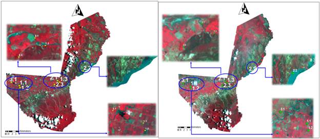
FIGURE 1 (a and b) (a) Fragment of the image Landsat 7 ETM of the year 2000, RGB: 432 and (b) Fragment of the image Landsat 8 OLI_TIRS of the year 2014, RGB: 543. 

Table 3 highlights the ecosystems and environmental services observed in the field and referred to the coordinate system at the points where they were observed in 2014, and it is appreciated that there are visual changes in most of them. Because there is no real evidence of contamination for the year 2000, it can be inferred that the evidence from 2014 constitutes the basis for assuming that these changes are primarily due to agricultural activities that influence the variations of the ecosystems appreciated.

TABLE 3 Ecosystems and environmental services observed in the field 

Ecosystem and Environmental Services	Points Referred to Image	Description	Location (Datum WGS84_19N)
			EAST	NORTH
Vegetation (1)	1.1	Crop (sugarcane)	305683	1054388
	1.2	Herbaceous Vegetation	305748	1053828
	1.3	Shrubs-Forests	317544	1055405
Water (2)	2.1	Motatán River Bank	316937	1055830
	2.2	Agua Viva Dam	324488	1058658
	2.3	Main Chanel (irrigation system)	316007	1054754
Soils (3)	3.1	Bare Soils	303333	1055342

In the same way, in 2018, coordinates were validated in the field referring to agricultural crops that were observed in the 2017 image, which according to ^{Duarte et al. (2017}), is used to correct a use map and / or to validate it. It is very remarkable a growth in the cultivated area, denoted by the appreciation of red color that shows the vegetation in the combination of bands (543), including areas that previous years were without any vegetation (bare). It was validated in field that they were being cultivated as it can be seen in figure 2.

FIGURE 2 (a and b) Fragment of the image Landsat 8 OLI_TIRS of the year 2017, RGB: 543. 

The analysis of the spatial distribution of the main ecosystems is carried out with the visual-digital method of interpretation of satellite images, for the years 2000, 2014 and 2017. The different coverage or classes (differentiated in the images) represent a signature by radiance values each of the bands. Then, the methods and tools used are described sequentially.

In the image fragments, differentiating the colors and tonalities, a layer of points was made in .shp format and 60 pixels were identified for each of the appreciable classes (resulting in seven differentiated classes). This process is carried out in each of the images (three years), in order to determine the classes for a later supervised classification of them. This classification constitutes the result of the temporal spatial characterization. With the pixels sampled in each class an output file is created in .gsg format, containing the spectral response (spectral signature) of the classes, it stores the statistical data of the classes in each of the bands. These statistical data were used to compare the classes and determine that there are significant differences between the means of the classes, using tools of inferential statistical comparison of samples; the software used for the analysis is STATGRAPHIS Centurion. If there are no differences, the process is repeated to determine the classes (resample the points to create the classes again), and, in this way, to make the spectral values precise, before performing the supervised classification.

A dendrogram (tree outline) is also generated in the ArcGIS 10.1 software for each created signature file (year 2000, 2014 and 2107) in a text file to see the differences and similarities between classes. This text file generates two components: the first component is a table of distances between pairs of classes, presented in the sequence for the fusion. The second component is a graphical representation of the classes, made with ASCII characters, which demonstrates the relationships and hierarchy of the fusion. The graph illustrates the relative distances between pairs of merged classes in the signature file, which are based on statistically determined similarities. The classes themselves represent clusters of cells or cells of training samples drawn from the study site. In this way, the potential of the merged classes is determined.

The dendrogram is validated with Fisher's Multiple Minimum Difference Test procedure (LSD), using the statistical software.

The classification method used was that of maximum likelihood on the set of the 3 raster bands aligned on both satellites, and it created an output raster with the specified classes. The tool takes into account the variances and covariances of the class signatures when it assigns each cell to one of the classes represented in the signature file, to then, make a visual comparison of the classified maps.

Seven classes will be contemplated for the classification. Class 1 corresponds to agricultural vegetation. Class 2 are soils with stubble or in preparation activities. They correspond to observations in the field, recorded with the GPS, of sugarcane plots that had been burned for the harvest, as well as "new" plots with recent logging activities (ready to be incorporated into agricultural crops). These two classes are closely related to agricultural activities. Class 3 corresponds to the vegetation of dense forest. Class 4 are bodies of water. Class 5 refers to infrastructures and floors provided with cover. They were considered as a single class because the colors and shades in different RGB combinations look similar. Classes 6 and 7 discriminate shadows and clouds, respectively.

RESULTS AND DISCUSSION

In correspondence with the methods described above, the results of the spatial-temporal comparison that is shown by a thematic representation of the main classes for each of the analyzed years is analyzed and discussed as shown in Figure 3.

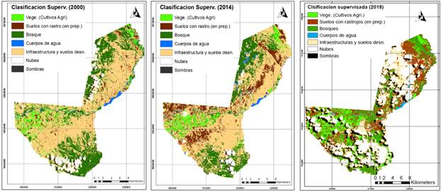
FIGURE 3 (a, b and c) (a) Supervised Classification of Miranda Municipality corresponding to the year 2000, (b) Supervised Classification of Miranda Municipality corresponding to the year 2014. (c) Supervised Classification of Miranda Municipality for the year 2017. 

Table 4 includes the amount of area classified for each class expressed in km² in the three resulting maps. The area of vegetation remains practically constant from 2000 to 2014 and, in the last three years, it has increased notably by 44.45 km², unlike bare soils (which reflect preparatory work), increased by approximately 37 km² in 2014 and in the following 39.35 km².

Greater area of water bodies is denoted for the years 2014 and 2017 because these two images present a greater amount of shadows that generate clouds and are confused with bodies of water. It is a somewhat erroneous result because of the confusion due to the similarity of the Spectral response in the pixels. That similarity is appreciated in each of the dates studied in the dendograms of the spectral classes. As regards the infrastructure class and completely bare soils, they show an increase of 1.18 km² approximately for 2014, which indicates urban, industrial and soil growth with erosion problems. In 2017 a considerable reduction is seen of 103.3 km², specifically for the occupation of these areas in agricultural crops and also to the overlap generated by the amount of clouds and shadows (class 6 and 7 respectively) in the image of 2017 (occupation that was validated in the field, specifically in these overlapping areas).

As for the areas of dense forest, there is a successive decrease of approximately 27.26 km² for the year 2017, which denotes a growth of the agricultural frontier. These variations, although in some of the classes are small, can have a reflection of the spatial variability and, at the same time, they are associated to the increase of the agricultural activity. The expansion of the agricultural frontier and the extraction of the forest resource, is what generally predominates in the studies of temporal space comparison related to the coverage or uses of land, and are directly associated with the dynamics of change of growth of the agricultural frontier (^{Bocco et al., 2001}; ^{Cabral, 2011}; ^{Orozco et al., 2015}; ^{Fragoso, 2017}).

TABLE 4 Result in terms of cells and areas of the temporal digital comparison (2000-2014) generated by the supervised classification with the spectral values 

	Year 2000		Year 2014		Year 2017
Classes	Área (km²)	(%) of surface that it represents	Área (km²)	(%)of surface that it represents	Área (km²)	(%)of surface that it represents
Vegetation (agricultural crops)	23.83	6.33	23.79	6.32	68.28	18.14
Bare soils with stubble (in preparation)	13.23	3.51	51.15	13.59	90.5	24.04
Forest	91.73	24.37	70.79	18.81	64.47	17.13
Bodies of water	6.71	1.78	6.76	1.8	9.84	2.61
Infrastructure and bare soils	208.85	55.48	210.03	55.8	107	28.43
Clouds	24.14	6.41	11.3	3	26.45	7.03
Shadows	7.93	2.11	2.59	0.69	9.88	2.62
TOTAL	376.42	100	376.42	100	376.42	100

CONCLUSIONS

The digital visual analysis referred to the spatial-temporal variability denotes the characteristics of environmental contamination product of an intensive agricultural activity, in the time of approximately 18 years. The measurable result in terms of area denotes a growth of 44.45 km² in agricultural areas for the year 2017, which corresponds to a decrease in forests of 27.26 km² and a decrease in the area designated as bare soils, specifically in the year 2107.

The image of 2014 presents a greater number of cells classified without clouds and shadows, so, it is more appropriate to take the information on bodies of water and infrastructure that does not show much variability over time, from this image. In that image, it is observed that the territory has populated areas, infrastructures supporting agricultural production (roads, warehouses, agro-industry, etc.), and eroded soils more than 55% and that the bodies of water practically remain constant and occupy approximately 1.79% of the municipality surface.

The information referring to the spectral characteristics of the different coverage in the area occupied by the municipality and those generated in the thematic maps, as well as the edaphoclimatic information, make up a small GIS of the environmental characterization of the municipality, being available for environmental plans.

REFERENCES

ALONSO DEL VAL, F.J.; COFIÑO, A.; FERNÁNDEZ, J.M.; FERRER, F.; FRANCÉS, E.; GUTIÉRREZ, J.M.; FERNÁNDEZ, B.; DOMÍNGUEZ, M.: “La Zonificación Agroecológica como mecanismo para potenciar la diversificación de la producción agrícola en Cantabria”, [en línea], En: III Congreso de la asociación Hispano-Portuguesa de Economía de los Recursos naturales y Ambientales, España, 2008, DOI: http://cifacantabria.org/Documentos/2008_ZONIFICACION%20AGROECOLOGICA_AERNA.pdf, Disponible en:Disponible en: http://cifacantabria.org/Documentos/2008_ZONIFICACION%20AGROECOLOGICA_AERNA.pdf , [Consulta: 5 de julio de 2017].

ARIZA, A.: “Descripción y Corrección de Productos Landsat 8 LDCM”, Knowledge Portal, UNSPIDER . Último acceso, 1, 2013.

BOCCO, G.; MENDOZA, M.; MASERA, O.R.: “La dinámica del cambio del uso del suelo en Michoacán: Una propuesta metodológica para el estudio de los procesos de deforestación”, Investigaciones geográficas, (44): 18-36, 2001, ISSN: 0188-4611.

CABRAL, F.: Dinámica espaciotemporal de uso del suelo en la UMAFOR 12 del Estado de México mediante el uso de sistemas de información geográfica (1990-2007), Universidad Autónoma Chapingo, thesis, Chapingo, Texcoco, Estado de México, México, 2011.

DUARTE, E.; ORELLANA, O.; MARADIAGA, I.; CASCO, F.; FUENTES, D.; JIMÉNEZ, A.; EMANUELLI, P.; MILLA, F.: Mapa Forestal y Cobertura de la Tierra de Honduras: Análisis de Cifras Nacionales, Honduras, 2017.

FRAGOSO, N.: Comparación del cambio de cobertura y uso de suelo a través de Sistemas de Información Geográfica en Acaxochitlán, Hidalgo, Universidad Veracruzana, M. thesis, Veracruz, México, 2017.

GÓMEZ GARCÍA, J.J.; SAMANIEGO, J.; ANTONISSEN, M.: Consideraciones ambientales en torno a los biocombustibles líquidos, ser. Serie Medio ambiente y desarrollo No 137, no. ser. 137, Ed. CEPAL, Santiago de Chile, Chile, 2008, ISBN: 978-92-1-323209-5.

MILANES, Y.: “Influencia de la mecanización agrícola en la contaminación ambiental. Universidad de Granma, Bayamo, Cuba [en línea] 2009, 2008”, [en línea], En: Universidad de Granma, 2009, Disponible en:Disponible en:http://www.monografias.com/trabajos-pdf/mecanizacion-agricola-contaminacion/mecanizacion-agricola-contaminacion.pdf , [Consulta: 30 de mayo de 2018].

MONTOYA, R.; GARCÍA, J.; PADILLA, J.: “Utilización de un SIG para la determinación del impacto ambiental generado por las actividades agrícolas, ganaderos e industriales: el caso de Zapotitlán en la reserva de la biosfera de Tehuacán Cuiclatán”, Boletin A.G.E, (38): 115-130, 2004.

OROZCO, M.C.; CERON, L.E.; MARTINEZ, J.P.; OSPINA, R.: “Análisis de los patrones espaciales del paisaje en un corredor biológico del macizo colombiano cauca.”, Biotecnología en el Sector Agropecuario y Agroindustrial: BSAA, 13(1): 54-63, 2015, ISSN: 1909-9959.

PINEDA, L.; SUÁREZ, J.: “Elaboración de un SIG orientado a la zonificación agroecológica de los cultivos”, Revista Ingeniería Agrícola, 4(3): 28-32, 2014, ISSN: 2306-1545, E-ISSN: 2227-8761.

PONVERT, D.D.; LAU, Q.A.: “Uso de las imágenes de satélites y los SIG en el campo de la Ingeniería Agrícola”, Revista Ciencias Técnicas Agropecuarias, 22(4): 75-80, 2013, ISSN: 1010-2760, E-ISSN: 2071-0054.

REYES, G.; CHAPARRO-GIRALDO, A.; ÁVILA, K.: “Efecto ambiental de agroquímicos y maquinaria agrícola en cultivos transgénicos y convencionales de algodón”, Revista Colombiana de Biotecnología, 12(2), 2010, ISSN: 0123-3475.

RODRÍGUEZ, H.; CERÓN-MUÑOZ, M.F.; PALACIO, L.G.; BEDOYA, G.I.: “Aplicación de los sistemas de información geográfica en la planificación de la asistencia técnica con enfoque territorial en cadena láctea”, Livestock Research for Rural Development, 27, 2015, DOI: http://www.produccion-animal.com.ar/produccion_y_manejo_pasturas/indice_verde/41-Aplicacion.pdf.

SHORTLE, J.S.; ABLER, D.G.: Environmental policies for agricultural pollution control, Ed. CABI, Departament of Agricultural Economics and rural Sociology Pensylvania State University, USA, 240 p., 2001, ISBN: 0‐85199‐3.

SMITH, A.M.; KOLDEN, C.A.; TINKHAM, W.T.; TALHELM, A.F.; MARSHALL, J.D.; HUDAK, A.T.; BOSCHETTI, L.; FALKOWSKI, M.J.; GREENBERG, J.A.; ANDERSON, J.W.: “Remote sensing the vulnerability of vegetation in natural terrestrial ecosystems”, Remote Sensing of Environment, 154: 322-337, 2014.

Received: February 15, 2018; Accepted: December 10, 2018

^*Author for correspondence: Lexa Dayana Pineda-Santos, e-mail: [e-mail]

Lexa Dayana Pineda-Santos, Ing. Agrícola, profesora, ULA-NURR, Villa Universitaria, La Concepción de Trujillo, Municipio Pampanito, Estado Trujillo, e-mail: [e-mail]

Jorge Eduardo Suárez-Hernández, e-mail: [e-mail]