Artículo original

Influence of temperature and composition on the prediction of the thermophysical properties of steel (I)

Influencia de la temperatura y la composición en la predicción de las propiedades termofísicas del acero (I)

0000-0003-2287-7519Yanan Camaraza-Medina^{1  *} 

¹Universidad de Matanzas. Matanzas, Cuba.

ABSTRACT

A proposal for the modeling of two thermo physical properties of steel as a function of the temperature and composition is presented. A residual method based on a progressive adjustment of functions is applied to estimate two thermo physical properties (electrical resistivity and linear thermal expansion) corresponding to 32 steels types with a composition (C, Mn , P, S, Si, Ni, Cr, Mo, V) and that operate in a temperature range from 0^oC to 800^oC. The validation and adjustment of the proposed models is made by comparing it with available experimental data. The weaker adjustment was achieved in the modeling of the electrical resistivity of AISI-SAE 405 steel with a mean and maximum deviation obtained of 8,2% and -9,9% respectively, while the best indices were obtained in the estimation of the density of AISI-SAE 1030 steel with a mean and maximum deviation obtained from 0,9% and 1,3% respectively. In all cases, the agreement of the proposed model is good enough to be considered satisfactory for practical design. Regarding the elements of study presented, there is no evidence of similar expressions in the available and known literature, which is why they are considered a scientific novelty.

Key words: Thermo physical properties; progressive adjustment method; experimental data generalization; mean absolute error

RESUMEN

Se presenta una propuesta para el modelado de dos propiedades termofísicas del acero en función de la temperatura y la composición. Se aplica un método residual basado en un ajuste progresivo de funciones para estimar dos propiedades termofísicas (resistividad eléctrica y dilatación térmica lineal) correspondientes a 32 tipos de aceros con una composición (C, Mn, P, S, Si, Ni, Cr, Mo , V) y que operan en un rango de temperatura de 0oC a 800oC. La validación y ajuste de los modelos propuestos se realiza comparándolos con los datos experimentales disponibles. El ajuste más débil se logró en el modelado de la resistividad eléctrica del acero AISI-SAE 405 con una desviación media y máxima obtenida de 8,2% y -9,9% respectivamente, mientras que los mejores índices se obtuvieron en la estimación de la densidad de acero AISI-SAE 1030 con una desviación media y máxima obtenida de 0,9% y 1,3% respectivamente. En todos los casos, la concordancia del modelo propuesto es suficientemente buena para considerarse satisfactoria para el diseño práctico. En cuanto a los elementos de estudio presentados, no existe evidencia de expresiones similares en la literatura disponible y conocida, por lo que se consideran una novedad científica.

Palabras-clave: propiedades termofísicas; método de ajuste progresivo; generalización de datos experimentales; error absoluto medio

Introduction

Currently, the high cost in money and time linked to experimental tests for the evaluation of thermo physical properties of steels, has established the preference for the use of predictive models in order to avoid this complex task (^{Şahinoğlu & Rafighi, 2021}).

When a large set of experimental data is available, artificial neural network (ANN) and finite element method (FEM) have been widely used in predictive modeling (^{Min, et al., 2020}). A detailed review of the available and known literature shows that currently reported methods for estimating thermo physical properties of steels, although they include dependence on composition and temperatures, only have the ability to predict a unitary property of the selected steel (^{Shi, et al., 2018}).

Using ANN, a model was created to predict the thermal conductivity of AISI-SAE1045 steel, establishing its dependence on temperature and composition. The prediction was based on a Bayesian statistical framework (^{Peet, Hasan & Bhadeshia, 2011}).

Other studies were focused on the prediction of three-dimensional heat flow, as well as heat transfer coefficient distributions in space and time. FEM techniques are used to study the phase transformation and its impact on the average heat transfer coefficient in the heat treatment of forged steels (^{Khodabakhshi & Kazeminezhad, 2011}; ^{Bouissa, et al., 2019}).

The dependence between the temperature and the mean heat transfer coefficient, as well as the cooling curves, the cooling rate curves and the distortion are predicted from the iterative modification of the concentrated heat capacity method and the heat transfer method. reverse heat in AISI-304 and AISI-1045 steels. To study the density variation of AISI-316L steel, the laser power, speed and scanning spacing were used during selective laser melting, using variance analysis for this purpose (^{Miranda, et al., 2016}).

Five different numerical algorithms, including Heat Balance Method (HBM), Revised Heat Balance Method (R-HBM), Nonlinear Beck Estimation Method (BEM), Inverse Finite Element Optimization Method (FIOM) and the finite element optimization method (FOM) were used for the prediction of thermal conductivity in carbon steels (^{Somasundharam & Reddy, 2020}).

Another work considers that the simultaneous estimation of the thermal conductivity is dependent on the temperature and the specific heat, assuming that this dependence is a parametric variation of the temperature, estimating the properties from the solution of the inverse problem (^{Wang & Adachi, 2019}). With this objective, it is established that the prediction models must take the composition as the only input data (^{Lieth, et al., 2021}).

Recently, a combined model was presented that includes the influence of composition and temperature on the variation of thermal conductivity in austenitic stainless steels (^{Narayana, et al., 2020}). Other methods, to perform prediction correlations, use a multiple linear regression analysis in the estimation of the thermal conductivity of carbon steels (^{Zheng, et al., 2020}). A similar study proposes a nonlinear regression equation to predict the cooling limit curve and thermal conductivity in carbon steels (^{Borisade, et al., 2021}). Other researchers, through the use of ANN, take the composition (Si, Cr, Ni, Mo) in alloyed steels as a starting point to estimate the cooling curve required in the heat treatment, also facilitating the evaluation of thermal conductivity (^{Xie, et al., 2021}).

Therefore, despite the existence of multiple investigative works on the subject, none of them presents a methodology that allows the prediction of an extended group of thermo physical properties of a wide range of steels, nor does it establish the dependence of these properties with composition and temperature, so the existence of a prediction method that resolves these limitations would be extremely useful (^{Gomez, et al., 2020}; ^{Li, et al., 2021}).

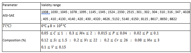
In this study, a prediction method based on the adjustment and validation of experimental data is presented through the mathematical application of the residual method based on the progressive adjustment of functions (PAF), which will allow estimating two thermo physical properties (electrical resistivity and linear thermal expansion) corresponding to 32 classes of steels with a composition (C, Mn, P, S, Si, Ni, Cr, Mo, V), operating in a temperature range from 0^oC to 800^oC.

Materials and methods

2.1 Data processing using the progressive adjustment method.

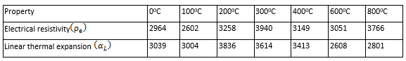
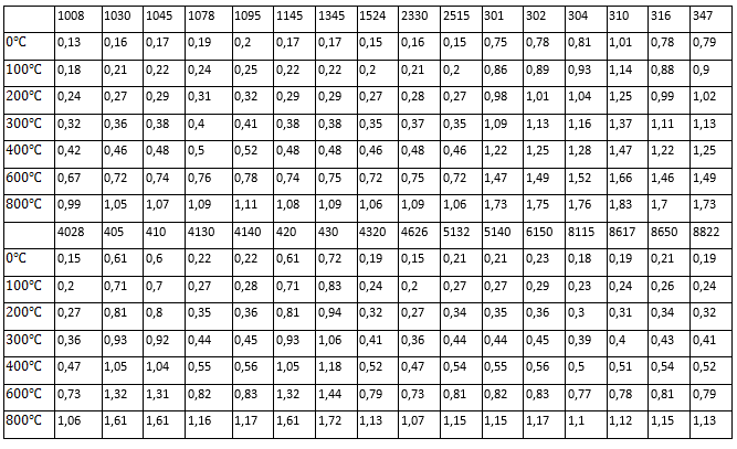
The available experimental data relate the influence of temperature and composition on the variation of the studied thermo physical properties. In collaboration with the School of Engineering and Applied Science, Khazar University (Azerbaijan), the experimental data used in the adjustment and validation of the models were obtained. Table 1 summarizes the number of available experimental data for each value of temperature and thermo physical property studied, while Table 2 summarizes the validity range of the proposed method.

Table 1 - Number of experimental data available. 

The modeling is carried out using the method of progressive function adjustment (APF). The analysis is too expensive and complex, and for reasons of space it cannot be fully shown here, however, as the applied procedure is identical for the two thermo physical properties, the modeling of the electrical resistivity will be detailed, while for the thermal expansion linear only the equations obtained, adjustments and validation will be given.

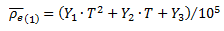
For electrical resistivity, once the experimental data has been grouped into the 32 AISI-SAE classifications covered (see table 2), the average value is obtained for each AISI-SAE steel and temperature range, using Equation 1.

Equation 1. Mean values calculations

where:

	is the average of the property or composition for each steel studied at temperature T.
	is the sum of all available values ​​of each property or composition in each steel studied at temperature T.
	is the number of samples available in each steel studied at temperature T.

The average values ​​obtained with Equation 1 are given in table 3, while table 4 summarizes the average composition per steel.

Table 2 - Validity range of the proposed method 

Table 3 Average values  

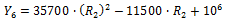
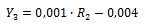
From the average composition (see table 4), the composition factors R ₁ y R ₂ , are determined, given in Equations 2 and 3, (^{Camaraza-Medina, Hernandez-Guerrero & Luviano-Ortiz, 2021}a).

Equation 2. Calculation of the composition factor R _1.

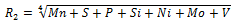
Equation 3. Calculation of the composition factor R ₂ .

In Equations 2 and 3, the composition values ​​are given in %.

Table 4 - Average composition values per steel studied, (%) 

AISI	1008	1030	1045	1078	1095	1145	1345	1524	2330	2515	301	302	304	310	316	347
C	0,08	0,31	0,47	0,78	0,98	0,46	0,41	0,22	0,33	0,15	0,13	0,13	0,07	0,23	0,07	0,08
Mn	0,4	0,7	0,75	0,45	0,39	0,84	1,72	1,49	0,69	0,49	1,89	1,89	1,89	1,89	1,89	0,4
P	0,03	0,03	0,03	0,03	0,03	0,03	0,03	0,03	0,03	0,03	0,03	0,03	0,03	0,03	0,03	0,03
S	0,04	0,04	0,04	0,04	0,04	0,06	0,03	0,04	0,03	0,03	0,02	0,02	0,02	0,02	0,02	0,04
Si	-	-	-	-	-	-	0,26	-	0,28	0,28	0,64	0,64	0,64	1,31	0,64	-
Ni	-	-	-	-	-	-	-	-	3,47	4,97	7	6,7	9,06	20,31	11,66	-
Cr	-	-	-	-	-	-	-	-	-	-	17,2	18,2	19,2	24	17	-
Mo	-	-	-	-	-	-	-	-	-	-	-	-	-	-	2,58	-
V	-	-	-	-	-	-	-	-	-	-	-	-	-	-	-	-
AISI	4028	405	410	4130	4140	420	430	4320	4626	5132	5140	6150	8115	8617	8650	8822
C	0,07	0,28	0,06	0,13	0,31	0,41	0,13	0,1	0,2	0,27	0,33	0,41	0,51	0,16	0,18	0,51
Mn	1,89	0,79	0,84	0,84	0,49	0,87	0,87	0,87	0,54	0,54	0,69	0,78	0,8	0,79	0,79	0,87
P	0,03	0,03	0,03	0,03	0,03	0,03	0,03	0,03	0,03	0,03	0,03	0,03	0,04	0,03	0,03	0,03
S	0,02	0,04	0,03	0,02	0,03	0,03	0,02	0,03	0,03	0,03	0,03	0,03	0,04	0,03	0,03	0,03
Si	0,64	0,28	0,77	0,77	0,28	0,28	0,86	0,86	0,24	0,23	0,28	0,28	0,28	0,23	0,28	0,28
Ni	10,66	-	-	0,61	-	-	-	0,61	1,8	0,83	-	-	-	0,29	0,53	0,53
Cr	18,2	-	13,3	12,7	0,98	0,98	13,2	17,2	0,52		0,9	0,8	0,98	0,42	0,52	0,52
Mo	-	0,26	-	-	0,21	0,21	-	-	0,26	0,21	-	-	-	0,12	0,2	0,2
V	-	-	-	-	-	-	-	-	-	-	-	-	0,13	-	-	-

The PAF method is generated from a base correlation, to which corrections are made through linear or polynomial functions (^{Camaraza-Medina, 2021}). To obtain the base correlation, the method of least squares is applied to the mean values ​​given in Table 3, obtaining a polynomial in the form 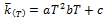per steel, (it can be used a linear function, but the predictive capacity of the model is reduced). Table 5 summarizes the parameters a, b and c for each correlation performed, the R ² , as well as the respective composition values R ₁ estimated with Equation 2, (see table 4 for the composition values ​​used).

Table 5 - Correlation of the mean values for the first adjustment. 

AISI- SAE	R 1	a	b	c	R ^2	AISI- SAE	R 1	a	b	c	R ^2
1008	0,283	0,095	41,52	14091	0,99	4028	0,529	0,091	40,32	14953	0,98
1030	0,557	0,086	47,92	15921	0,98	405	3,651	0,042	86,95	55697	1,0
1045	0,686	0,092	44,02	16995	1,0	410	3,576	0,032	96,9	56147	0,99
1078	0,883	0,094	42,82	18111	1,0	4130	1,136	0,083	43,69	22128	1,0
1095	0,99	0,088	45,84	19613	1,0	4140	1,179	0,075	49,62	20897	0,98
1145	0,678	0,089	42,05	16385	1,0	420	3,646	0,035	110,2	64742	1,0
1345	0,64	0,09	41,58	16017	1,0	430	4,155	0,029	117,0	68638	1,0
1524	0,469	0,079	51,61	15273	0.98	4320	0,849	0,089	44,06	18114	1,0
2330	0,57	0,089	41,5	16158	1,0	4626	0,52	0,09	40,23	14862	0,98
2515	0,387	0,091	38,74	13655	1,0	5132	1,109	0,087	42,15	20947	0,99
301	4,162	0,008	112,0	74737	1,0	5140	1,1	0,08	45,67	22131	0,99
302	4,28	0,009	110,5	74678	0,99	6150	1,221	0,086	48,9	22192	0,99
304	4,387	0,006	112,5	73855	1,0	8115	0,762	0,089	43,05	17217	1,0
310	4,922	-0,019	115,8	92523	1,0	8617	0,837	0,089	43,96	17985	1,0
316	4,132	0,01	96,59	76428	0,99	8650	1,015	0,088	46,18	1988	1,0
347	4,274	0,017	94,7	75535	0,98	8822	0,866	0,089	44,27	18296	1,0

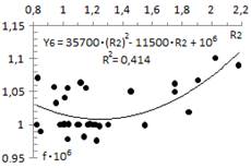
To establish the base function in the prediction of electrical resistivity, all the values a, b and c are individually correlated with R ₁ (see table 5), thus obtaining a first approximation to describe the dependence between temperature and thermal conductivity, for any of the AISI-SAE steels evaluated. The correlations obtained are graphically represented in Fig 1 , 2, 3.

Fig 1 - Correlation between c and the factor R ₁  

Fig. 2 - Correlation between b and the factor R ₁  

Fig. 3 - Correlation between c and the factor R ₁  

Correlations plotted in Fig 1, 2 and 3 are given by:

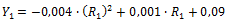
Equation 4. Obtaining the adjustment parameter 1 of the APF.

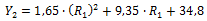
Equation 5. Obtaining the adjustment parameter 2 of the APF.

Equation 6. Obtaining the adjustment parameter 3 of the APF.

The function taken for the first progressive adjustment was a second order polynomial; therefore, Equations 4, 5 and 6 can be summarized in Equation 7:

Equation 7. Calculation of electrical resistivity in the first approximation.

Equation 7 is the first approximation or base function of the progressive function adjustment. To carry out the second step of the adjustment, the values ​​of are calculated using equation 7 for each interval shown in Table 3 and subsequently a quotient is established with the experimental values, thus defining the required setting value. Mathematically this is described by Equation 8:

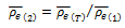
Equation 8. Calculation of the adjustment residual value for the second round of APF.

The results obtained with the use of equation 8 are summarized in table 6.

Table 6 - Values per steel. 

AISI- SAE	00C	1000C	2000C	3000C	4000C	6000C	8000C
1008	1,106	1,103	1,098	1,093	1,088	1,082	1,077
1030	1,056	1,064	1,071	1,073	1,072	1,057	1,043
1045	1,032	1,036	1,038	1,039	1,039	1,039	1,039
1078	0,992	0,991	0,995	1,0	1,006	1,017	1,025
1095	1,0	1,001	1,003	1,004	1,005	1,006	1,007
1145	1,0	1,001	1,002	1,003	1,004	1,006	1,007
1345	1,0	1,001	1,002	1,003	1,004	1,006	1,007
1524	1,083	1,091	1,097	1,101	1,095	1,066	1,035
2330	1,065	1,05	1,039	1,032	1,026	1,02	1,011
2515	0,999	1,001	1,002	1,003	1,004	1,006	1,007
301	1,091	1,068	1,071	1,068	1,062	1,04	1,013
302	1,049	1,038	1,034	1,034	1,03	1,015	0,995
304	1,003	1,002	1,003	1,003	1,002	0,993	0,979
310	1,053	1,031	1,017	1,001	0,987	0,98	0,939
316	1,101	1,088	1,061	1,05	1,02	0,984	0,96
347	1,068	1,025	1,011	1,011	0,993	0,98	0,957
4028	1,0	1,001	1,002	1,003	1,004	1,006	1,007
405	0,94	0,947	0,947	0,953	0,95	0,959	0,964
410	0,976	0,984	0,992	0,996	1,0	0,994	0,985
4130	1,043	1,019	1,001	0,988	0,98	0,969	0,964
4140	0,969	0,968	0,97	0,97	0,968	0,954	0,944
420	1,101	1,109	1,117	1,119	1,125	1,124	1,111
430	1,001	1,013	1,031	1,03	1,054	1,083	1,079
4320	1,0	1,001	1,002	1,004	1,005	1,006	1,007
4626	1,0	1,001	1,002	1,003	1,004	1,006	1,007
5132	1,004	0,985	0,974	0,969	0,967	0,967	0,97
5140	1,053	1,038	1,027	1,006	0,992	0,976	0,968
6150	1,001	1,002	1,003	1,004	1,005	1,007	1,007
8115	1,0	1,001	1,002	1,003	1,004	1,006	1,007
8617	1,0	1,001	1,002	1,004	1,005	1,006	1,007
8650	1,001	1,002	1,003	1,004	1,005	1,006	1,007
8822	1,0	1,001	1,002	1,004	1,005	1,006	1,007

In table 6, using the method of least squares, a correlation is obtained in the form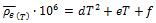 for each steel. Table 7 summarizes the parameters d, e and f for each correlation and their R ² values, as well as the R ₂ factors estimated using Equation 3, (see table 4 for the composition per steel). To define the second correction (see table 7), the values d, e and f are individually correlated with R ₂ . The obtained fits are provided in Fig 4, 5 and 6.

Table 7 - Correlation of the mean values for the second adjustment. 

AISI- SAE	R 2	d	e	f	R^2	AISI- SAE	R 2	d	e	f	R ^2
1008	0,828	0,016	-50,82	1106737	1,00	4028	1,088	-0,006	14,21	999539	1,00
1030	0,937	-0,137	89,91	1056883	0,96	405	1,137	-0,002	29,34	941683	0,94
1045	0,952	-0,022	24,74	1032956	0,97	410	1,227	-0,113	101,3	975850	0,98
1078	0,849	0,017	32,4	989545	0,98	4130	1,01	0,156	-218,2	1040832	0,99
1095	0,824	-0,006	13,22	1000325	1,00	4140	1,092	-0,066	20,6	968398	0,97
1145	0,982	-0,006	13,64	999799	1,00	420	1,155	-0,112	102,8	1100620	0,98
1345	1,194	-0,006	13,87	999710	1,00	430	1,245	-0,076	168,3	997889	0,95
1524	1,118	-0,22	112,8	1083341	0,98	4320	1,305	-0,006	13,45	1000070	1,00
2330	1,456	0,079	-125,7	1063315	0,99	4626	1,169	-0,006	14,19	999549	1,00
2515	1,552	-0,007	14,66	999362	1,00	5132	1,007	0,135	-142,9	1000587	0,95
301	1,759	-0,058	-40,37	1083664	0,95	5140	1,028	0,101	-192,4	1055817	0,99
302	1,745	-0,042	-26,99	1044803	0,97	6150	1,036	-0,006	13,14	1000755	1,00
304	1,847	-0,065	24,53	1001557	0,99	8115	1,105	-0,006	13,64	999913	1,00
310	2,203	0,035	-157,9	1048715	0,97	8617	1,168	-0,006	13,26	1000081	1,00
316	2,025	0,045	-221,1	1105170	0,99	8650	1,18	-0,005	12,98	1000428	1,00
347	1,908	0,11	-207,0	1057128	0,94	8822	1,199	-0,005	13,23	1000135	1,00

Fig. 4 Correlation between d and the factor R ₂  

Fig. 5 Correlation between e and the factor R ₂  

Fig. 6 Correlation between f and the factor R ₂  

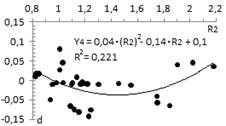
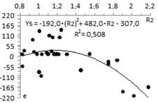
The correlations plotted in Figures 4, 5 y 6 are given by:

Equation 9. Obtaining the adjustment parameter 4 of the APF.

Equation 10. Obtaining the adjustment parameter 5 of the APF.

Equation 11. Obtaining the adjustment parameter 6 of the APF.

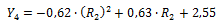
The function taken for the second progressive adjustment was a second order polynomial, therefore, Equations 9, 10 and 11 can be summarized in Equation 7:

Equation 12. Calculation of electrical resistivity in the second approximation.

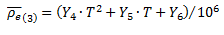
The electrical resistivity can then be estimated from the product of the two progressive adjustments made, (Equations 7 and 12), obtaining that:

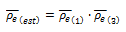
Equation 13. Calculation of the estimated electrical resistivity.

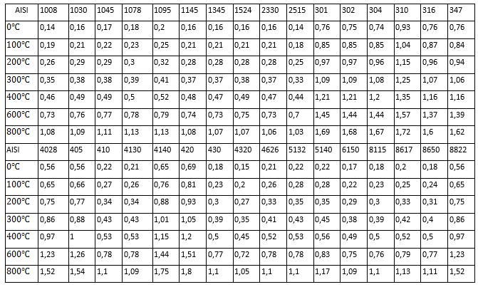
The electrical resistivity values ​​computed using Equation 13 are given in the table 8.

Table 8 Values  

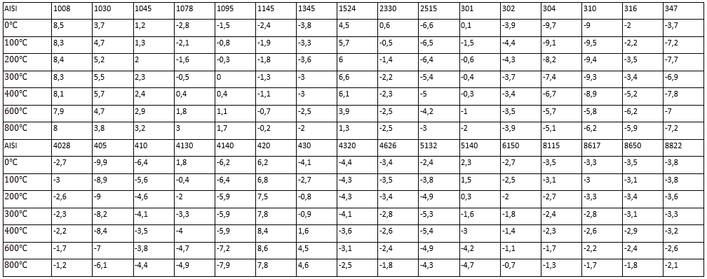
The percentage of deviation (error) computed with the proposed method is obtained through Equation 14 (^{Camaraza-Medina, Guerrero-Hernandez & Luviano-Ortiz, 2021}b):

Equation 14. Calculation of the correlation error of the proposed method (Equation 13).

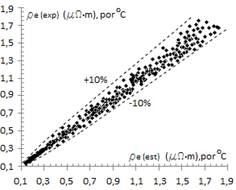
Table 9 summarizes values obtained by comparing the experimental data tabulated in Table 3 with the results obtained through Equation 14. Figure 7 correlates the values with an error band of 10%.

Table 9 - Values obtained in the correlation of experimental data. 

Fig. 7 Correlation of  

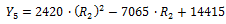
Applying a procedure analogous to the electrical resistivity, a methodology is established to estimate linear thermal expansion, which is given by Equations 15, 16, 17, 18, 19, 20, 21 and 22:

Equation 15. Obtaining the adjustment parameter 1 of the APF.

Equation 16. Obtaining the adjustment parameter 2 of the APF.

Equation 17. Calculation of linear thermal expansion in the first approximation.

Equation 18. Obtaining the adjustment parameter 3 of the APF.

Equation 19. Obtaining the adjustment parameter 4 of the APF.

Equation 20. Obtaining the adjustment parameter 5 of the APF.

Equation 21. Calculation of linear thermal expansion in the second approximation.

Equation 22. Calculation of the estimated linear thermal expansion.

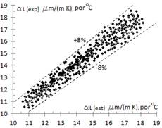
In the figure 8, valuesare correlated with an error band of 8%.

Fig. 8 - Correlation of  

Results and discussion

Estimation of the dispersion obtaining in the APF method application.

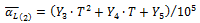
Table 10 gives the values of maximum error and mean absolute error (MAE) obtained by correlating Equations 13 and 22 with the available experimental data. The MAE values are estimated from Equation 23, (^{Camaraza-Medina, et al., 2020}):

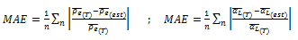
Equation 23. Estimation of the MAE values.

For the electrical resistivity, the most unfavorable dispersion index is obtained for AISI-SAE 405 steel, with a 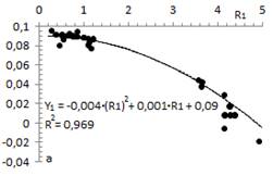of -9.9% at a temperature of 100oC and an MAE of 8.2% in the 81.9% of available experimental data. The best fit is achieved in the correlation of the properties of AISI-SAE 1095 steel, with a 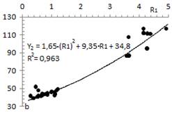of 1.7% at a temperature of 800^oC, with an MAE of 0.8% in the 85.1% of the available experimental data.

In the linear thermal expansion modeling, the most unfavorable dispersion index is obtained for AISI-SAE 1524 steel, with a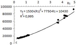of 7.0% at a temperature of 400^oC and an MAE of 6.1% in the 79.6% of the available experimental data. The best fit is achieved in the correlation of the properties of AISI-SAE 1030 steel, with a of 1.3% at a temperature of 400oC and an MAE of 0.9% in the 83.4% of the available data.

Table 10 Values y MAE obtained in the correlation with experimental values. 

Conclusions

A predictive method is presented to estimate the electrical resistivity and linear thermal expansion in 32 types of steels with a known composition (C, Mn, P, S, Si, Ni, Cr, Mo, V) and operating in temperature ranges from 0oC to 800oC. The proposed models were verified by comparison with available experimental data.

In the electrical resistivity modeling, the most unfavorable dispersion index is obtained for AISI-SAE 405 steel, with a of -9.9% at a temperature of 100oC and an MAE of 8.2% in the 81.9% of available experimental data. The best fit is achieved in the correlation of the properties of AISI-SAE 1095 steel, with a of 1.7% at a temperature of 800^oC, with an MAE of 0.8% in the 85.1% of the available experimental data. In the linear thermal expansion modeling, the most unfavorable dispersion index is obtained for AISI-SAE 1524 steel, with aof 7.0% at a temperature of 400^oC and an MAE of 6.1% in the 79.6% of the available experimental data. The best fit is achieved in the correlation of the properties of AISI-SAE 1030 steel, with a of 1.3% at a temperature of 400^oC and an MAE of 0.9% in the 83.4% of the available data.

In all cases, the agreement of the proposed model with the available experimental data is good enough to be considered satisfactory for practical design. Regarding the elements of the study presented, there is no evidence of similar expressions in the available and known literature, for this reason, the proposal presented is considered as a scientific novelty in the field of knowledge addressed.

References

Borisade, S.G., Ajibola, O.O., Adebayo, A.O., & Oyetunji, A. (2021). Development of mathematical models for the prediction of mechanical properties of low carbon steel (LCS).Materials Today: Proceedings, 38, 1133-1139.

Bouissa, Y., Shahriari, D., Champliaud, H., & Jahazi, M. (2019). Prediction of heat transfer coefficient during quenching of large size forged blocks using modeling and experimental validation.Case Studies in Thermal Engineering, 13, 100379.

Camaraza-Medina, Y., Sanchez-Escalona, A.A., Retirado-Mediaceja, Y., & García-Morales, O.F. (2020). Use of air-cooled condenser in biomass power plants: a case study in Cuba. International Journal of Heat and Technology, 38(2), 425-431.

Camaraza-Medina, Y. (2021) Methods for the determination of the heat transfer coefficient in air cooled condenser used at biomass power plants, International Journal of Heat and Technology , 39(5), 1443-1450.

Camaraza-Medina, Y., Hernandez-Guerrero, A., & Luviano-Ortiz, J.L. (2021a). New method for the cost assessment analysis of shell-and-tube heat exchangers. Latin American Applied Research, 51(4), 315-320.

Camaraza-Medina, Y.,Hernandez-Guerrero, A., & Luviano-Ortiz, J.L. (2021b). New Improved Method for Heat Transfer Calculation Inside Rough Pipes. Journal of Heat Transfer- ASME, 143(7), 074503.

Gomez, C.F., van der Geld, C.W.M., Kuerten, J.G.M., Bsibsi, M., & van Esch, B.P.M. (2020). Quench cooling of fast-moving steel plates by water jet impingement.International Journal of Heat and Mass Transfer, 163, 120545.

Khodabakhshi, F., & Kazeminezhad, M. (2011). The effect of constrained groove pressing on grain size, dislocation density and electrical resistivity of low carbon steel. Materials & Design, 32, 3280-3286.

Li, W., Chen, H., Li, C., Huang, W., Chen, J., Zuo, L., & Zhang, S. (2021). Microstructure and tensile properties of AISI 321 stainless steel with aluminizing and annealing treatment.Materials & Design , 205, 109729.

Lieth, H.M., Al-Sabur, R., Jassim, R.J., & Alsahlani, A. (2021) Enhancement of corrosion resistance and mechanical properties of API 5L X60 steel by heat treatments in different environments. Journal of Engineering Research, 9(4B), 428-440.

Min, K.M., Jeong, W., Hong, S.H., Lee, C.A., Cha, P.R., Han, H.N., & Lee, M.G. (2020). Integrated crystal plasticity and phase field model for prediction of recrystallization texture and anisotropic mechanical properties of cold-rolled ultra-low carbon steels.International Journal of Plasticity, 127, 102644.

Miranda, G., Faria, S., Bartolomeu, F., Pinto, E., Madeira, S., Mateus, A., & Carvalho, O. (2016). Predictive models for physical and mechanical properties of 316L stainless steel produced by selective laser melting.Materials Science and Engineering: A,657, 43-56.

Narayana, P.L., Lee, S.W., Park, C.H., Yeom, J.-T., Hong, J.-K., Maurya, A.K., & Reddy, N.S. (2020). Modeling high-temperature mechanical properties of austenitic stainless steels by neural networks. Computational Materials Science,179,109617.

Peet, M.J., Hasan, H.S., & Bhadeshia, H.K.D.H. (2011). Prediction of thermal conductivity of steel.International Journal of Heat and Mass Transfer ,54(11-12), 2602-2608.

Şahinoğlu, A., & Rafighi, M. (2021) Investigation of tool wear, surface roughness, sound intensity, and power consumption during hard turning of AISI 4140 steel using multilayer-coated carbide inserts. Journal of Engineering Research , 9(4B), 377-395.

Shi, L., Lin, S.T.K., Lu, Y., Ye, L., & Zhang, Y.X. (2018). Artificial neural network based mechanical and electrical property prediction of engineered cementitious composites. Construction and Building Materials, 174, 667-674.

Somasundharam, S., & Reddy, K.S. (2020). Inverse analysis for simultaneous estimation of temperature dependent thermal properties of isotropic materials.Thermal Science and Engineering Progress, 20, 100728.

Wang, Z. L., & Adachi, Y. (2019). Property prediction and properties-to-microstructure inverse analysis of steels by a machine-learning approach.Materials Science and Engineering: A , 744, 661-670.

Xie, Q., Suvarna, M., Li, J., Zhu, X., Cai, J., & Wang, X. (2021). Online prediction of mechanical properties of hot rolled steel plate using machine learning.Materials & Design , 197, 109201.

Zheng, B., Shu, G., Wang, J., Gu, Y., & Jiang, Q. (2020). Predictions of material properties in cold-rolled austenitic stainless steel tubular sections.Journal of Constructional Steel Research, 164, 105820.

Received: May 14, 2022; Accepted: June 24, 2022

^*Autor para correspondencia. E-mail: [e-mail]

El autor declara no tener conflictos de intereses.

El autor participó en el diseño y redacción del trabajo, y análisis de los documentos.