ARTÍCULO ORIGINAL

 

Information analysis of pattern and randomness

 

Análisis de información en patrones y aleatoriedad

 

 

Ernesto Estévez-Rams^1*, Edwin Rodríguez Horta¹, Beatriz Aragón Fernández², Pablo Serrano Alfaro¹, Raimundo Lora Serrano³

¹Facultad de Física-Instituto de Ciencias y Tecnología de Materiales(IMRE), Universidad de la Habana, San Lazaro y L. CP 10400. La Habana. Cuba.
²Universidad de las Ciencias Informáticas (UCI), Carretera a San Antonio, Boyeros. La Habana. Cuba.
³Universidade Federal de Uberlandia, AV. Joao Naves de Avila, 2121- Campus Santa Monica, CEP 38408-144, Minas Gerais, Brasil.

*Autor para la correspondencia: [e-mail]

 

 

---

ABSTRACT

Complex patterns are ubiquitous in nature and its emergence is the subject of much research using a wide range of mathematical tools.  On one side of complexity lies completely periodic system, and in the other side random behavior, both trivially simple from a statistical point of view. A fingerprint of complexity is the existence of large spatio-temporal correlations in the system dynamics. In this contribution, we will review two threads in complexity analysis, both steaming from information theory: Lempel-Ziv analysis of complexity, and computational mechanics. We discuss the usefulness of both approaches through the analysis of several examples. A first system will be the spatio-temporal evolution of cellular automata where transfer of information can be quantified by Lempel-Ziv measures. A second example will be random walk with bias and persistence; computational-mechanics will prove adequate for assessing the amount of wandering vs the patterned movement of the walker. Finally, disorder and pattern forming in layer crystal structure will be analyzed. Wrapping up, some discussion on the general nature of the examples analysis will be carried pointing to the appropriateness of the developed tools for studying the computational processing capabilities of complex systems

Key words:complexity, information, Lempel-Ziv, computational mechanics.

---

RESUMEN

Los patrones complejos son comunes en la naturaleza y su surgimiento es objeto de mucha investigación utilizando una amplia gama de herramientas matemáticas. A un lado de la complejidad se encuentra la repetición completamente periódica, y en el otro, lo totalmente aleatorio, ambos trivialmente simples desde el punto de vista estadístico. Una huella dactilar de la complejidad es la existencia de correlaciones temporales o espaciales de largo alcancen la dinámica de los sistemas. En esta contribución, revisaremos brevemente dos métodos de realizar el análisis de la complejidad, ambos derivados de la teoría de la información: a través de la aleatoriedad de Lempel-Ziv y utilizando la mecánica computacional. La utilidad de ambas aproximaciones será discutida a través del análisis de varios ejemplos.  Un primer sistema será la evolución espacio temporal de autómatas celulares, donde la transferencia de información será cuantificada utilizando Lempel-Ziv. Un segundo ejemplo será el del caminante aleatorio con sesgo y persistencia, la mecánica computacional demostrará ser apropiada para determinar la cantidad de deambular versus el movimiento predictible del caminante. Finalmente, desorden y formación de patrones en estructuras de capas será analizado. Para terminar, se discute la naturaleza general del análisis, insistiendo en la utilidad de las herramientas presentadas para el estudio de las capacidades de procesamiento computacional de los sistemas complejos.

Palabras clave: complejidad, información, Lempel-Ziv, mecánica computacional.

---

 

 

INTRODUCTION

Trivial initial conditions can give rise to complex patterns, and this has been the subject of intensive studies (See (Crutchfield, 2012) and reference therein). Complexity arises in the modeling of large systems in broad areas of science such as those found in physics, chemistry or biology. It is clear that periodic behavior is far from complex as it can be modeled with few variables and the nature of the information is extremely redundant. However, it is also agreed, that completely random processes are also not complex. In spite of its heavy information content, randomness is easily modeled as a simple coin throw experiments shows. Complexity lies between these two extremes and a fingerprint of its occurrence is the presence of large spatio-temporal correlations (Wolfram, 1986).

A way of looking into complexity is to ask the ability of a dynamical system to generate and store information. Viewed from this perspective, they can be seen as computational machines that generates symbols. The study of the system is then reduced to quantify how it is capable of such computing capacity, which, in turn, can be relevant if it is intended to tune the control parameters of the system to take advantage of its computing ability (Crutchfiled, 2012).

Kolmogorov, or algorithmic complexity, has been at the root of complexity analysis. Kolmogorov complexity characterize a system by the length of the shortest algorithm running on a Universal Turing Machine (UTM), capable of reproducing the system (Kolmogorov, 1965; Li, 1993).  A periodic system will need a very short algorithm to be reproduced, while a completely random system can only be replicated by describing it to the smallest detail. Kolmogorov complexity is then not a true measure of complexity but of randomness, its absolute nature, up to a constant value, exhibits useful properties (in what follows we will use the more appropriate term of Kolmogorov randomness). The main drawback of Kolmogorov randomness, as a practical tool, is its non-computability because of the halting problem (Li, 1993). This limitation has driven researchers to define practical alternatives, based on the compressibility of the mathematical description of the system. All these alternatives are merely upper bounds to the true Kolmogorov randomness of the system.

The analysis usually involves characterizing the system configurations by its compressibility, where some compression software such as gzip or bzip2 is used (Dubaq, 2001). The use of compression software to estimate Kolmogorov randomness has a number of issues, one being the necessarily finite size of the words dictionary (Weinberger, 1992). This leads to limitations in the size of the systems analyzed, depending precisely in the Kolmogorov randomness of the sequence, the very quantity aimed to be estimated.

Lempel-Ziv complexity (Lempel, 1976) (from now on LZ76 complexity), closely related to Kolmogorov randomness, is a measure defined over a factorization of a character sequence. Data sequences from different sources have been analyzed by LZ76 complexity (Aboy, 2006; Chelani, 2011; Contantinescu, 2006; Liu, 2012; Rajkovic, 2003; Szczepanski, 2004; Talebinejad, 2011; Zhang, 2009). All analysis using LZ76 complexity are based on a theorem proved by Ziv (Ziv, 1978) that showed, that the asymptotic value of the LZ76 complexity growth rate (LZ76 complexity normalized by n/log n, where n is the length of the sequence) is related to the entropy rate h (as defined by Shannon information theory) for an ergodic source. Entropy rate has a close relationship with Kolmogorov randomness (Calude, 2002), and measures the irreducible randomness of a system (Feldman, 2008).

Consider an optimal computational machine capable of statistically reproducing the system dynamics. Optimality is understood as the simpler machine with best predictive power. Such machine is called ɛ-machine and its design, or its reconstruction from the available data, is the goal of computational mechanics (Crutchfield, 1992; Crutchfield, 2012).  Complexity analysis is then, using the epsilon-machine, to discover the nature of patterns and to quantify them. It is rooted in information theory concepts, and has found applications in several areas (Varn, 2013; Ryabov, 2011; Haslinger, 2010).  Its use in statistical mechanics, allowed to define and calculate magnitudes that complement thermodynamic quantities. One of such magnitude is the statistical complexity Cm, defined as the Shannon entropy over the probability of the causal states. A causal state is a set of pasts that determines probabilistically equivalent futures (Shalizi, 2001).  Entropy rate hm, already mentioned when describing the LZ76 complexity can also be calculated from the e-machine description of the system (Crutchfield, 2003). Finally, the excess entropy E, defined as the mutual information between past and future, and can be interpreted as the amount of memory needed to make optimal predictions, without taking into account the irreducible randomness (Feldman, 1998).

In this contribution, we will be reviewing the use of LZ76 and computational mechanics in the study of complexity. We will do so by dwelling into various examples: studying the spatio-temporal evolution of cellular automata (CA), quantifying the amount of wandering and purposely movement in a random walk with bias and persistence and finally, the emergence of disorder and pattern in layer structured crystals.

The paper is organized as follows. It first begins by mathematically introducing the various concepts already mentioned, which will also allow to fix notation. This will be followed by the discussion of the cellular automata dynamics. The next section will deal with the biased persistent random walk model and then the results for layer crystals will be presented. A discussion of the usefulness of the developed tools for studying the computational processing capabilities of complex systems will be made. Conclusions then follow.

The results presented in this paper have been partially published separately by the authors in (Estevez, 2015; Rodriguez, 2016a; Rodriguez, 2016b)

 

MATHEMATICAL BACKGROUND

A. Kolmogorov based normalized information distance

The Kolmogorov randomness K(s) of a string s, is the length of the shortest program s* that when run in a Universal Turing Machine (UTM), gives as output the string
 K(s) = |s*|.

Using UTM makes the Kolmogorov randomness an absolute measure, up to a constant factor. It is clear that a constant string can be described by a very short program, while a random string, say out of a coin toss experiment, will have not algorithmic way to be exactly predicted except by reproducing the string itself. The conditional Kolmogorov randomness K(s|p) can be introduced as the length of the shortest program that, knowing p, allows to compute s. Also, the joint Kolmogorov randomness K(s,p) is the size of the smallest program that computes both strings s and p. Without going into details, in what follows the allowed programs will be prefix-free, where no program is a proper prefix of another program (Li, 1993).  The halting program makes Kolmogorov randomness non-computable, which turns out to be a huge limitation for its practical use.

It can be shown that the following relation holds

K(s,p) K(s)+K(p|s*) = K(p)+K(s|p*) ,      (1)

where denotes that equality is valid up to a constant value independent of p and s.

Entropy density can be estimated from

The entropy rate is defined by

where H[s(1,N)] is the Shannon block entropy (Cover, 2006) of the string

In spite of the non-computability of the Kolmogorov randomness, the entropy density can be computed, as we do not need the actual K but only its scaling behavior.

The information about s contained in p is defined by

 I(s:p)=K(s)-K(s|p*),                (4)

which implies that I(s:p)=I(p:s) up to a constant.

Li et al. (li, 2004) defined the normalized information distance (NID) between two sequences s and p by the relation:

where, without loss of generality, it is assumed that K(p) > K(s).  NID is an information-based distance that quantifies how correlated are two sequence from the algorithmic perspective.  If two sequences can be, to a large extent, derived one from the other by a small sized algorithm, then the corresponding NID is small.

The problem with the use of equation (5) is that Kolmogorov randomness is non computable, the practical alternative is to estimate dNID from

where C(x) is the compressed size of the string x. Compression have been made using available software such as gzip or bzip2 (Li, 2004; Emmert, 2010), with no significant difference between the different compression softwares.

Instead of using a compression algorithm, if s and p have the same length, then we rewrite equation (6) in terms of the entropy density

h(x) is, contrary to K(x) a computable magnitude and this is the approach will be using.

B. Lempel-Ziv factorization and complexity

Let us call s(i,j) the substring of s starting at the position i and having length j. Define the operator

s(i,j)π = s(i, j-1)
π is kind of a drop operator, consequently,
s(i,j)π ^k = s(i, j-k).

The Lempel-Ziv factorization F(s) of the string s of length N is given by
F(s) = s(1, l₁)s(l₁+1, l₂)... s(l_m-1+1, N),

where there are m factors such that each factor s(l_k-1+1, l_k) complies with

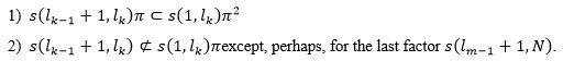
The partition F(s) is unique for every string (Lempel, 1976).

For example, the exhaustive history of the sequence u = 111010100011 is F(s) = 1.110.10100.011,
where each factor is delimited by a dot.

The LZ76 randomness C_LZ(s) of the string s, is the number of factors in Lempel-Ziv factorization. In the example above, C_LZ(s) = 4.

In the limit of very large string length, CLZ(s) is bounded by (Lempel, 1976)

which allows to define a normalized LZ76 randomness as

Ziv(Lempel y Ziv, 1976) proved that, if s is generated by an ergodic source, then where h(s) is the entropy rate defined above in equation (3). This allows to use cLZ(s) as an estimate of h(s) for N>>1. dNCD can then be computed using the estimates of entropy rate given by equation (3), we will denote such distance by d_LZ.

C. Computational mechanics: Casual states, statistical complexity, entropy rate and excess entropy

We will be mostly following (Shalizi, 2001). Consider a process that produces as output a (bi) infinite sequence of characters, drawn from a given alphabet Σ. Take a particular realization of the process with output string s, which will be partitioned in two , the past, and , the future. Assuming that strings are drawn from a distribution, possibly unknown, then two , that conditions the same probability for all futures , are said to belong to the same causal state Cp. By construction, the set of causal state (denoted by {Cp} of size |{Cp}|) uniquely determines the future of a sequence which allows to define a function ε over , relating to its causal state Cp.

The statistical complexity is defined as the Shannon entropy over the causal states

The logarithm is usually taken in base two and the units are then bits. The set of causal states is related to the optimal memory required for prediction; more memory resources will not improve the predictive power of the process. Statistical complexity, being the Shannon entropy over the causal states, is therefore a measure of how much memory the system needs to optimally predict the future.

The entropy rate, can be calculated as

We will be considering first order Markov process, where the excess entropy is given by

Excess entropy is a measure of the resources needed, once the irreducible randomness has been subtracted (Feldman, 2008).

When the size of the alphabet Σ is finite, the number of causal states for the first order Markov process is also finite, and the dynamics of the system can be optimally described by a finite state machine (FSM), which in this case will represent the ε-machine. 

The ε-machine FSM can be described by a digraph, where each node corresponds to a causal state and the directed transitions between nodes are labeled as sk|P(Cm|Cp). sk is the emitted symbol, while making a transition from Cp to Cm the arriving state is uniquely determined by the emitted symbol, a property called unifiliarity.

The reader can refer to (Shalizi, 2001; Feldman, 1998) for further discussion.

Information transfer in the spatio-temporal evolution of cellular automata

Our first systems will be discrete time and space cellular automata (CA), which has been the subject of intense research over the past decades ((Kari, 2005) and reference therein). CA can go from periodic patterns to universal computing capabilities (Wolfram, 1984). This last behavior is amazing, as a CA can be specified by a finite number of local rules acting over a finite number of states. In spite of the local nature of the rules, CA can achieve large spatio-temporal correlations (Wolfram, 1986).

We will define, for the purposes of this article, a one dimensional CA, as a tern (Σ, s, Φ), where Σ is, as defined before, a finite alphabet; s = s0s1...sN-1 is a set of sites and; Φ is a local rule. If s^t = s^t0,s^t1,s^t2,...s^tN-1 denotes a particular configuration of the sites values at time t, then

 s^t+1i  = Φ[ s^t-1i-r, s^t-1i-r+1,...,s^t-1i+r].

For elementary CA (ECA), r = 1, and a binary alphabet Σ = {0, 1} is used.

There are a total of 256 possible rules for ECA which can be labeled by a number. To each rule Φ, a label R is assigned according to a scheme proposed by Wolfram that has become standard (Wolfram, 02):

 R = Φ(0,0,0)2⁰+Φ(0,0,1)2¹+Φ(0,1,0)2²+... +Φ(1,1,1)2⁷.

ECA rules can be partitioned into equivalence classes as a result of mirror and reversion symmetries, the analysis of the rules can then be reduced to a representative member of each class. CA have been classified in a number of ways (Kari, 2005), where the most cited one is the original classification of Wolfram (Wolfram, 1984). Starting from an arbitrary random initial configuration, CA are classified as:

W1: configurations evolves to a homogeneous state;
W2: configurations evolves to a periodic behavior;
W3: configurations evolves to aperiodic chaotic patterns;
W4: configurations evolves to configurations with complex patterns and long lived, correlated localized structures.

Wolfram classification is vague; as a result, the assignment of each rule to a Wolfram class is ambiguous.

In (Estevez, 2015) how ECA rules transfer information from the (random) initial configuration as they evolve was studied. The d_LZ between two consecutive configurations st and st+1 was computed for successive values of time t.  After dropping the first 2000 steps, the d_LZ values were averaged (denoted as dp_LZ) and plotted against the final entropy density (Figure 1).  Three clusters were identified, one with the d_LZ values around 1, labeled dp3. A second cluster, dp2, was made of rules belonging to W2, and a third cluster, with zero d_LZ, made of W1 rules and labeled dp1. Group of rules in dp1 have a complete transfer of information as the configurations evolves, and these rules also show entropy densities near zero. The group of rules dp2 span the whole range of entropy density values, but show dp_LZ distance between 10^-3 and 10^-1, they also show a trend of decreasing dp_LZ  with increasing entropy density. The third group of rules dp3 loose, on the average, all information from one-time step to the next.

In addition, the effect of changing the initial configurations was considered. Two initial sequences were taken, the second one with a single (random) site changed with respect to the first one. Then both ECA were left to evolve and the d_LZ between them were calculated at each time step. This was done 1000 times for each rule and the results averaged.  Different behaviors were discovered from almost no sensibility to the perturbation of the initial condition, to heavy dependence on the initial condition as shown in Figure 2.

Rules 150 as well as 60, 90 and 105 (and equivalents) behaves in a very interesting way. Figure 3 shows the distance between the non-perturbed and perturbed evolution for rule 150. The fractal nature of the behavior is clear and can be understood by looking into the difference map. The reiterative collapse of the d_LZ curve to almost zero value, can be pointed in the difference map to the apex of the triangle regions.

Analysis of random walk viewed as a symbol generating process.

We turn to a one-dimensional random walker (RW) which was studied by the authors in (Rodriguez, 2016). The walker is allowed to move to the right, or to the left, a unit length in a unit time. The probability that the walker chooses right will be a control parameter labeled by r. p, on the other hand, is the probability that the walker keeps moving in the same direction as the previous step. r, es also known as bias, and p as persistence. Also, a probability l that the walker makes no move at a given step is allowed.  The set of control parameters is then (r, p, l) which will be taken fixed in time.

Our process knows outputs values from the set , the first symbol representing a move to the right, the second symbol no move, and the last symbol a move to the left. The control parameters (probabilistically) decide the next move based on the previous one, and therefore the dynamics of the system can be described by a first order Markov process.  The most FSM describing this process for different values of the control parameters are shown in figure 4. It was found that the most unpredictable dynamics happens at r = l = 1/3 with an entropy density of h = log₂3 = 1.5849 bits/site.

From the ε-machine is straightforward to calculate the entropy density and excess entropy as a function of the control parameters. Such diagrams allows asserting the amount of movement, which can be considered random (wandering), in contrast to the movement following some pattern. This kind of information is not directly available through usual statistical physics analysis. Figure 5 shows such diagrams.

Excess entropy is a measure of patterned movement. As latency increases the walker stays longer runs in the same place (state ) and the patterned movement goes to zero. For a given value of latency, persistence controls the patterned movement. Small, or near one, values of persistence results in larger patterned movement. The relation with bias is less straightforward and seems less sensitive to this control parameter. Complementary, entropy density shows a maximum around {r,p}={1/2,1/2} for a fixed latency value. Entropy density is witnessing the wandering movement of the walker. The movement for small values of persistence is patterned, but the system alternates between three states. If latency is small, the movement gets closer to an antiferromagnetic order and the walker does not get far from its initial position, the drift velocity is near zero. The reduction of drift velocity is not consequence of wandering movement, but of its patterned alternate character.   As persistence increases, still with small latency, the excess entropy decreases as a result that the system has longer runs on the state. Once persistence goes above one half, excess entropy starts climbing and the dynamics gets increasingly closer to ferromagnetic order.

Ising models for the study of stacking disorder in layered crystals: ε-machine analysis.

Close packed structures are special type of layer structures ubiquitous in nature. The close packed condition is referred to the constrain that two consecutive layers with the same lateral displacement, are forbidden.  Two periodic arrangements that differ only on their stacking order are termed to belong to the same polytypic family and each member of a family is called a polytype. Experimentally it has been found that perfect periodic stacking are the exception, usually stacking disorder is present in varying degrees from low density to almost complete disruption of any underlying order.  If the stacking ordering in CPS is coded as some binary code, then it is possible to study, polytypism and stacking disorder, by writing the Hamiltonian that describes the interaction between the binary codes, treated as spins (Uppal, 1980; Kabra, 1988; Shaw, 1990).

When considering only finite range interaction, a large class of system can be cast in the framework of the Ising model, which has a Hamiltonian of the type:

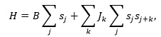
As usual, B described an external field intensity, Jk is the interaction parameter for range k and si is the spin (pair of layers) at site i.  Now the system reduces to a dynamical system, typical in complexity analysis, where, because of the different interaction terms, patterns and disorder can arise witness by the resulting string of characters.

ε-machine analysis of Ising models have been studied before (Feldman, 1998). As in the case of the random walker, the process can be cast into a first order Markov process, in this case by using the transfer matrix formalism.  A FSM description of the system arises. The FSM of maximum connectivity is shown in Figure 6 together with the statistical complexity contour map, for a second neighbor interaction.

The complexity map directly describes the phase diagram. The appearance of different polytypes comes as result of the J1/J2 ratio. Phase transformation in this type of system is considered to be result of the parameters J1, J2, depending on external factors, such as temperature or pressure. Also, the ε-machine description allows to discover the polytypes appearing at the boundary between stable phases. Such calculation was performed for all boundaries in the phase diagram and Table I shows the polytypes at the FCC-DHCP border whose probability of occurrence is above 10%.

 

DISCUSSION AND CONCLUSIONS

Complexity analysis has a long story of development, still grasping what we mean by complex behavior has turned out to be a very complex problem. Perhaps there is no single definition for complexity; yet, it can be agreed, for a number of systems, that the emergence of new behavior from seemingly simple rules, when a large number of variables are involved, can be a fingerprint of complexity. If the systems can be mathematized as codes or strings of a numerable alphabet, then complexity is tractable from a number of angles. In this paper, we have explored two venues, which have proven useful in a number of cases. Computational mechanics, pioneered by Crutchfield and coworkers, is reaching a point of maturity were increasing practical applications can be fore-visioned. One of the outstanding aspect of computational mechanics is that it has allowed to explore in a quantitative and deep way the “quality” of disorder and pattern. In its framework the meaning of entropic measures such as entropy rate, excess entropy and statistical complexity have been clarified. It is also a practical tool. It uses in the analysis of layer solids just scratch the surface of its usefulness.

Although much less worked than computational mechanics, Lempel-Ziv has its own beauties. It is very practical; it allows to estimate entropy density from raw data if enough observations are made. If combined with ideas from Kolmogorov complexity it can be used to define empirical metrics over system dynamics. We have shown the power of Lempel-Ziv based analysis of CA spatio-temporal evolution. The method used is readily extendable to other systems in a straightforward manner.

ACKNOWLEDGMENTS

This work was partially financed by FAPEMIG under the project BPV-00047-13. EER which to thank PVE/CAPES for financial support under the grant 1149-14-8. Infrastructure support was given under project FAPEMIG APQ-02256-12. EDRH and PSA which to thank MES for master degree support.

 

REFERENCIAS BIBLIOGRÁFICAS

M. Aboy, R. Homero, D. Abasolo, and D. Alvarez. Interpretation of the Lempel-Ziv complexity measure in the context of biomedical signal analysis. IEEE Trans. Biom. Eng., 2006, 53, p. 2282–2288.

C. S. Calude. Information and Randomness, 2002, Springer Verlag.

A.B. Chelani. Complexity analysis of co concentrations at a trafc site in Delhi. Transp. Res. D, 2011, 16, p. 57–60, 2011.

S. Contantinescu and L. Ilie. Mathematical Foundations of Computer Science, 2006, 4/62. Springer Verlag, Berlin.

T. M. Cover and J. A. Thomas. Elements of information theory. 2006, Second edition. Wiley Interscience, New Jersey.

J. P. Crutchfield. Knowledge and meening ... chaos and complexity. In L. Lam and V. Narodditsty, editors, Modeling complex phenomena, 1992, Springer, Berlin, p.66–101.

J. Crutchfield and D. P. Feldman. Regularities unseen, randomness observed: Levels of entropy convergence. Chaos, 2003, 13, p.25–54.

J. P. Crutchfield. Between order and chaos. Nature, 2012, 8, p.17–24.

[Dubaq, 2001] J.-C Dubacq, B. Durand, and E. Formenti. Kolmogorov complexity and cellular automata classification. Th. Comp. Science, 2001, 259, p. 271–285.

F. Emmert-Streib. Exploratory analysis of spatiotemporal patterns of cellular automata by clustering compressibility. Phys. Rev. E, 2010, 81, p. 026103–026114.

E. Estevez-Rams, R. Lora-Serrano, C. A. J. Nunes, and B. Aragón Fernández, Lempel-Ziv complexity analysis of one dimensional cellular automata, Chaos 2015, 25, p.  123106-123116.

D.P. Feldman. Computational mechanics of classical spin systems. (1998)

D.P. Feldman, C.S. McTeque, J.P. Crutchfield, Chaos, 2008, 18, p. 043106.

R. Haslinger, K. L. Klinker, and C. R. Shalizi. The computational structure of spike trains. Neural computation, 2010, 22, p. 121–157.

J. Kari. Theory of cellular autoamta: A survey. Th. Comp. Science, 2005, 334, p. 3–33.

V. K. Kabra and D. Pandey, 1988, 61, p. 1493.

A. Lempel and J. Ziv. On the complexity of finite sequences. IEEE Trans. Inf. Th., 1976, IT-22, p. 75–81.

M. Li and P. Vitanyi. An Introduction to Kolmogorov Complexity and Its Applications. Springer Verlag, 1993.

M. Li, X. Chen, X. Li, B. Ma, and P. M. B. Vitanyi. The similarity metric. IEEE Trans. Inf. Th., 2004, 50, p.3250–3264.

L. Liu, D. Li, and F. Bai. A relative lempelziv complexity: Application to comparing biological sequences. Chem. Phys. Lett., 2012, 530, p.107–112.

A. N. Kolmogorov. Three approaches to the concept of the amount of information. Probl. Inf. Transm. (English Trans.)., 1965, 1, p.1–7.

M. Rajkovic and Z. Mihailovic. Quantifying complexity in the minority game. Physica A, 2003, 325, p. 40–47.

E. Rodriguez-Horta , E. Estevez-Rams , R. Lora-Serrano , B. Aragon-Fernandez, Correlated biased random walk with latency in one and two dimensions: Asserting patterned and unpredictable movement, Physica A, 2016, 458, p. 303312.

E. Rodriguez-Horta , E. Estevez-Rams , R.Neder, R. Lora-Serrano, Computational mechanics of stacking faults with finite range interaction: layer pair interaction, in press.

V. Ryabov, D. Neroth, Chaos, 2011, 21, p. 037113.

C. R. Shalizi and J. P. Crutchfield. Computational mechanics: pattern and prediction. J. Stat. Phys., 2001, 104, p. 817–879.

J. J. A. Shaw and V. Heine, J. Phys.: Condens. Matter., 1990, 2, p.4351.

J. Szczepanski, J. M. Amigo, E. Wajnryb, and M. V. Sanchez-Vives. Characterizing spike trains with lempel-ziv complexity. Neurocomp., 2004, 58-60, p. 77–84.

M. Talebinejad and A.D.C. Chanand A. Miri. A lempelziv complexity measure for muscle fatigue estimation. J. of Electro. and Kinesi., 2011, 21, p. 236–241.

M. K. Uppal, S. Ramasesha, and C. N. R. Rao, Acta Cryst. 1980, A36, p. 356.

D. P. Varn, G. S. Canright, and J. P. Crutchfield. ε-machine spectral reconstruction theory: a direct method for inferring planar disorder and structure from x-ray diffraction. Acta Cryst. A, 2013, 69, p.197–206.

M. J. Weinberger, A. Lemepl, and J. Ziv. A sequential algorithm for the universal coding of finite memory sources. IEEE Trans. Inf. Th., 1992, 38, p. 1002–1014.

S. Wolfram. Universality and complexity in cellular automata. Phys. D, 1984, 10, p. 1–35.

S. Wolfram. Theory and applications of cellular automata. 1986, World Scientific Press, Singapur.

S. Wolfram. A new kind of science. 2002, Wolfram media Inc., Champaign, Illinois.

Y. Zhang, J. Hao, C. Zhou, and K. Chang. Normalized Lempel-Ziv complexity and its applications in biosequence analysis, J. Math. Chem., 2009, 46, p. 1203–1212.

A. Lempel and J. Ziv, On the complexity of finite sequences, IEEE Trans. Inf. Theory 1978, 22, 75–81.

J. Ziv. Coding theorems for individual sequences. IEEE Trans. Inf. Th., 1978, IT-24, p. 405–412.

 

 

Recibido: 15/06/2016
Aceptado: 10/10/2016