


Mi SciELO
 Servicios personalizados
Servicios Personalizados
Revista

Articulo
 Español (pdf)
 Articulo en XML
 Referencias del artículo
 Enviar articulo por email
Indicadores
-
 Citado por SciELO
Links relacionados
-
 Similares en
SciELO
Similares en
SciELO
Compartir

 Permalink
Ingeniería Energética
versión On-line ISSN 1815-5901
Energética vol.36 no.1 La Habana ene.-abr. 2015
TRABAJO TEORICO EXPERIMENTAL
Solution to Carson's integrals through power series
Solución de las integrales de Carson mediante series de potencia
Ph.D José Alberto Gutiérrez Robles, MSc. Jorge Luis García Sánchez, Ph.D Pablo Moreno Villalobos, MSc. Verónica Adriana Galván Sánchez, MSc. Julian Sotelo Castañon, MSc. Eduardo Salvador Bañuelos Cabral
Universidad de Guadalajara (UdG), Mexico.
ABSTRACT
The problem ofelectromagnetic waves propagation inoverhead transmissionlines has apparently not been solved in a sound manner yet. While the problemdoes not have anexact analyticalsolutionwhen considering the presence of the actual surface of theearth, its approximate solutionintroducingtheoreticalsimplificationsis of formidable practical interest. Using quasi-static approximations Carson obtained integral equations to calculate the electromagnetic field due to a horizontal current carrying wire which is above a lossy ground plane. Carsonhimselfproposedthe first solutionto theseexpressions using power series expansions which does not possess uniform convergence andsincethen there have beenefforts toget a bettersolution. In this sense two clear approaches have been essentially followed. The first one consists on modifying the integrand in such a way that an analytic solution can be obtained. The second one is based on using numerical integration schemes.
Key words: ground returns impedance, carson's integrals, aerial transmission line, power series.
RESUMEN
El problema de la propagación de ondas electromagnéticas en líneas de transmisión aéreas aún no ha sido resuelto de manera definitiva. Si bien el problema no posee una solución analítica exacta cuando se considera la presencia de la superficie real de la tierra, su solución aproximada, introduciendo simplificaciones teóricas es de gran interés práctico. Usando aproximaciones cuasi-estáticas, en 1926 Carson obtuvo ecuaciones integrales para el cálculo del campo electromagnético generado por la corriente de un conductor horizontal sobre un plano de tierra imperfecto. La primera solución la propone el mismo Carson utilizando expansiones en series, las cuales no poseen convergencia uniforme y desde entonces se han hecho esfuerzos por tener una mejor aproximación. Se han seguido dos enfoques claros, el primero consiste en introducir modificaciones en el integrando de manera que sea posible obtener una solución analítica. El segundo, se basa en la utilización de métodos de integración numérica.
Palabras clave: impedancia de retorno por tierra, integrales de Carson, líneas de transmisión aérea, series de potencia.
Methodology: Because Carson integrals have adecreasing exponential term, the infinite upper limit can be substituted by a finite limit without altering the result beyond a preset error. With such limit substitution and using power series a new analytic solution with uniform convergence for all cases is obtained in this work.
For comparison purposes Carson´s series and approximated compact formulas published elsewhere are used. As a gold standard the numerical solution of Carson's integral using Romberg integration with an error of 10-21 is used.
Findings: The final results verify that the proposed solutions converge for all test cases, unlike Carson's formulas, and are more accurate than compact expressions.
Originality: It is developed a new way to solve Carson's integrals analytically.
INTRODUCTION
For the case of an aerial line; his geometry, the constructed material, the earth resistivity and the involved frequency, determines the line electrical parameters, means, the series impedance (Z) and the transversal admittance (Y). Due to the little earth transversal electrical field penetration, it is use to neglect the earth effect in the admittance, so the capacitance and the conductance are calculated under the assumption that the line is over a perfect infinite conductor plane. By the other hand, it is well known that the line series impedance is compound by three terms [1], written in equation (1) as,
Where: ZG is the geometric impedance which is calculated using the magnetic field extern to the conductors. ZC is the conductor's internal impedance, which models the effect of the longitudinal electric field inside the conductors. ZE is the earth impedance, which models the effect of the magnetic fields penetration inside the earth.
From the three terms of equation equation (1), Carson's integrals are the base of the earth impedance calculus [2]. In this work it is developed a new solution for these integrals and evaluates the solutions gives by the Carson series [2], approximate compact formulas [3] and the numerical solution [4-5]. There are some standards for ground considerations as [6-7], so, there are some works based on this works as [8-9], others using trunked series as [10] and another's ones using similar criteria as for the numerical solution of the Pollaczek's integral, as in [11-12]. This work is organized as follows: first we enounce the knowing Carson series, and then we analyze the solution by using approximate formulas. We follow with the proposed solution through power series, and then we make a qualitative analysis of the Carson's integrals to finish in the analysis of the results and conclusions.
CARSON SERIES
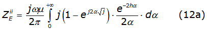
Considering a uniform line (the line material and the surrounding dielectric are homogeneous) and neglecting the displacement current, the self and mutual earth impedance described in the Carson integrals are [2], as it is described in equations (2a) and (2b).
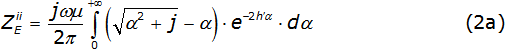
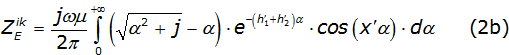
Where: µ is the air permeability; hi'=hi(√ωμσ) with 0,1 ≤hi≤ 200 like the i-esime conductor height; xi'=xi(√ωμσ) with 0,1 ≤xi≤ 1 000 like the distance between conductors; ω=2πf with 1x10⁻³ ≤f≤ 1x10⁸ like the frequency and 1x10⁻⁴ 1x10⁻¹ is the earth conductivity.
Defining the Carson's integral [3], given by equation (3),
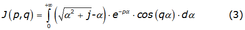
for the self-impedance p and q are defined by equations (4a) and (4b) as,
and for the mutual-impedance by equations (5a) and (5b),
being Φ=√ωμσ; h the conductor height and x the distance between conductors.
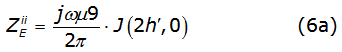
So, equation (2a) and equation (2b) could be written as equations (6a) and (6b) respectively,
Let it be define, p and θ, by equations (7a) and (7b) as,
Carson's integrals given by equation (3) could be separated in real and imaginary parts as [3], it is denoted by equation (8a) as,
With P and Q given, in terms of p and θ, by equations (8b) and (8c), respectively,
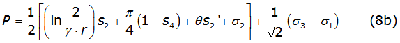
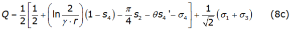
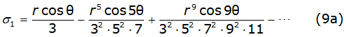
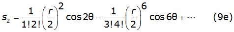
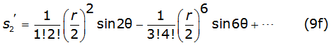
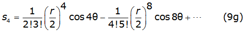
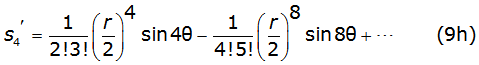
Into equation (8b) and equation (8c), γ is the Euler's constant and thes k and σk are the Carson's series terms [2], given by equations (9a), (9b), (9c), (9d), (9e), (9f) (9g) and (9h) as follows,


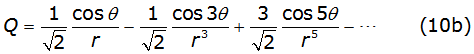
Carson's series converge to the right solution in the case of r<<5, in other case Carson propose the solution written in equations (10a) and (10b) [2],

The crossing from one solution (equation (8b) and equation (8c)) to other (equation (10a) and equation (10b)) is almost arbitrary and until now nobody has determined the exact way to do it. Even more there are intervals in which none of these formulas give adequate solutions.
SOLUTION BY APPROXIMATE FORMULAS
The process to obtain approximate formulas lies in the substitution of the term [(√(α2+j))-α] inside the Carson's integral by a function with similar behavior with analytical solution. The proposed function, by Derry et.al. is mentioned in equation (11) as follows [3],
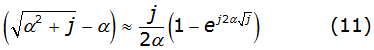
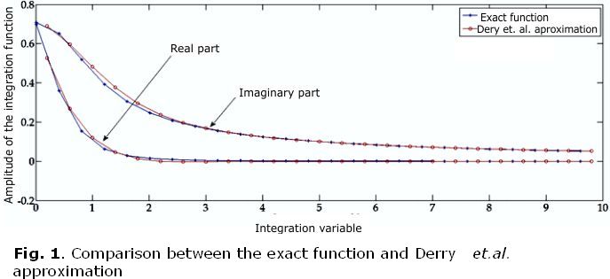
It is shown in figure 1, the comparison between the original integrand (from equation (3)) and the proposed one (from equation (11). It could be able to note that the approximate function will be a good solution only if the value is really big.
By substituting the proposed function into equation (2a) and equation (2b), it is obtained equations (12a) and (12b) as,
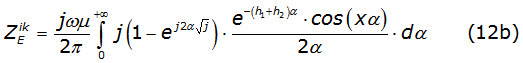
These equations have a well-known analytical solution denoted by equations (13a) and (13b), [3],
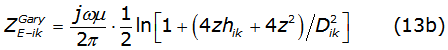
where: z=k/φ and Dik=√(hi+hk)2+x2 with k=1/√j.
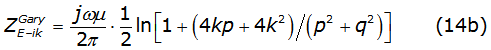
The self and mutual impedance like a function of p and q are given by equations (14a) and (14b) respectively,
SOLUTION TO CARSON'S INTEGRALS THROUGH POWER SERIES

It is developed an approximate new analytical solution to the Carson's integrals through power series. The first step to obtain this solution is the algebraic separation of equation (3) into two parts as is written in equation (15):

Then the radical is expressed as a Newton binomial expansion, but this radical doesn't have uniform convergence so previously the integral is separated into two parts to obtain equation (16),
Now, for each case one has the solutions given by equations (17a) and (17b) respectively,
Substituting equation (17a) and equation (17b) into equation (16), one obtains a series of integrals with a general form denoted by equation (18),
with n=0,2,4,6,… and m=1,-1,-3,-5,…. Constants kl and cl are calculated with equation (17a) and equation (17b) respectively.
Self-Impedance
To the self-impedance one has q=0, so equation (16) takes the algebraic structure of equation (19),
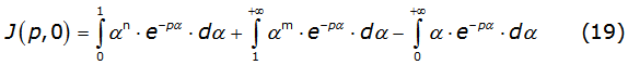
with n=0,2,4,6,… and m=1,-1,-3,-5,….
I. First integral
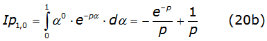
The first integral of equation (19) is solved with the recurrence equation (20a)
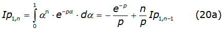
with , and the first integral solution given by equation (20b)
II. Second integral
The second integral is separated into three parts denoted by equation (21),

with m = -3, -5,...
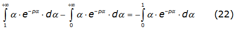
From this integral; the first integral of the right side is grouped with the third integral of equation (19)) to obtain one integral with the same mathematical structure as equation (20a) with n = 1, this is denoted by equation (22) as follows:
This integral is solved as equation (20a) with n = 1, means is equal to Ip1,1. Now, by substituting the superior limit by αmax, the second integral of equation (21) is solved by using the power series of e-pα to obtain equation (23) as,

This process generates a sequence of integral with the mathematical structure given by equation (24)
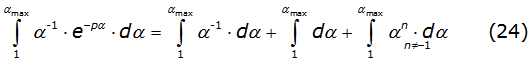
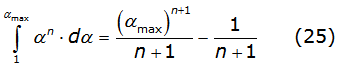
The first two integral of the right side of equation (24) are solved directly; the third one is solved with the recurrence relation denoted by equation (25),
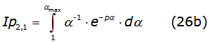
To complete the solution of the self-impedance, one need to solve the third integral of the right side of equation (21); this is performed by using the recurrence relationgiven in equation (26a),
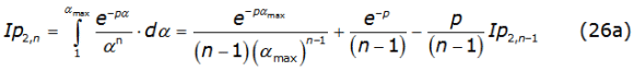
with n=2,3,4,..., where Ip2,1 is denoted in equation (26b) as,
Notice that equation (26b) has the same mathematical structure than equation (23).
Mutual-Impedance
For the mutual-impedance the equation (16) takes the structure given by equation (27) as,
with n = 0,2,4,6,… and m = 1,-1,-3,-5,….
I. First integral
The first integral of equation (27) is solved with the recurrence equation (28a),
with n = 2,3,4,… and the first two integrals given by equations (28b) and (28c),


II. Second integral
The second integral of equation (27) is separated into three parts given by equation (29) as,
with m = -3,-5,…. Now, the first integral of the right side of equation (19) is grouped with the third integral of equation (27) to obtain equation (30),
This integral is solved as equation (28c).
Now, by changing the superior limit by αmax, the third integral of equation (29) is solved with the following recurrence equation for n = 2,3,4,…. to obtain equations (31a) and (31b),
To solve equation (31a) and equation (31b), it is necessary to solve the following two integrals where Ip2,1 is equal to the second integral of equation (29) given by equation (32a) and Ia2,1 is given by equation (32b) respectively,
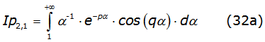
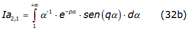
The integrals denoted by equation (32a) and equation (32b) are solved by using the power series of e-pα as it is written in equation (33a) and equation (33b),
The algebraic manipulation of these integrals conduce to equations (34a) and (34b),


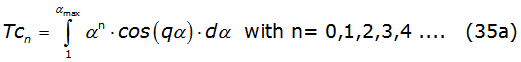
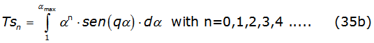
The second integral of equations (34a) and (34b) generate integrals with the mathematical structure denoted by equations (35a) and (35b),
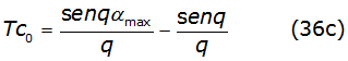
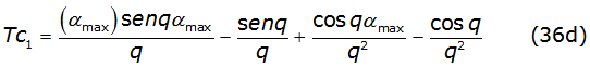
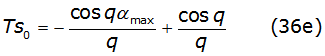
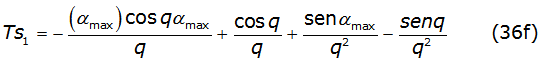
The recurrence relations to solve these equations are given by equations (36a) and (36b) respectively,
The first two terms of each recurrence relation are written in equations (36c), (36d), (36e) and (36f) as,
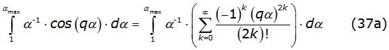
The first integral of equation (34a) and equation (34b) are solved by using the power series ofcos(qα ) and sin(qα), so one arrives to equations (37a) and (37b) as follows:
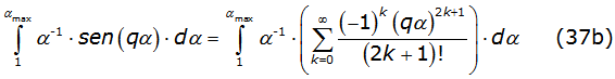
The power series of trigonometric functions don't have uniform convergence; this means that they don't have convergence for every limit; in this case they have convergence only when one has qα≤2 . When the argument of the trigonometric function doesn't comply with this restriction, it is necessary to modify the expressions; this process yields to equations (38a) and (38b),
In equation (38a) and equation (38b), n is an integer such that n corresponds to q value to obtain the condition nπ≤αmax≤(n+1)π. The next step is to move the functions into the interval in which converge restrictions are reaching it, so one obtains equation (39a) and (39b) respectively,
Now, the power series of the trigonometric functions are used; initially it is taken the first integrals from equation (39a) and from equation (39b) to obtain equations (40a) and (40b),
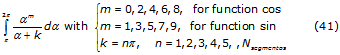
These integrals are solved directly; then the power series are substituted in the rest of the integrals to obtain new integrals with the mathematical structure given by equation (41),
The generalized solution for even m is denoted by equation (42a),
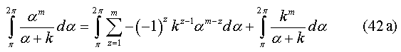
By the other hand, the generalize solution for odd m is denoted by equation (42b),
Like this, one has an analytical new solution for the Carson's integrals through power series.
QUALITATIVE ANALYSIS OF CARSON'S INTEGRALS
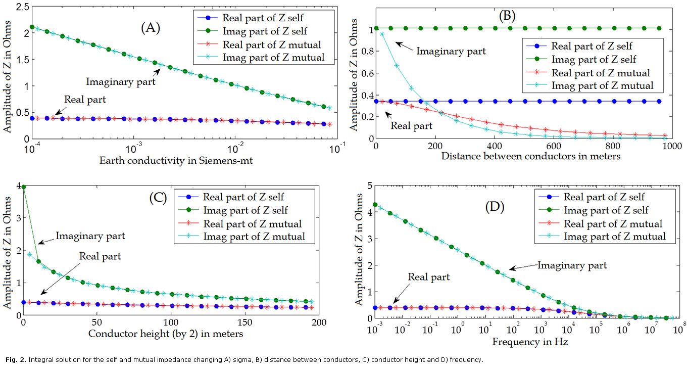
To realize the analysis of the Carson's integrals behavior, these are solved by the Romberg integration method. These solutions will be the point of reference, it is important to note that the numerical implementation is a rigid solution in which one used millions of points if it is necessary to have the preset error, for this reason sometimes the process is slow but in every case one obtain a very trust full solution. Initially one takes the four variable parameters which are fixed to one value, then one varies just one of them to obtain the results showed in figures 2a, 2b, 2c and 2d. The fixed values (base values) arehij = 40, xij = 5, f = 60 and σ = 0,01.
From the results showed in figure 2 one could deduce that every single parameter makes that Z value changes in different way, so to take into account the combined effect of these parameters, it is used the p and q variables of the Carson's integrals and all the combinations are referred to these variables. One specific combination ofhij, xij, f and gives like a result some values of p and q; to take into account all possible variations inside the established intervals according with equation (2a) and (2b) it is obtained the minimum and maximum values of p and q given by equations (43a), (43b), (43c) and (43d) as follows,
The previous equations indicate that it could be possible to evaluate the effect of the variations ofhij, xij, f and σ in the entire established interval by using the variation of p and q from their minimums to their maximums. To realize the analysis in base on p and q it could be notice that these values are connected each other because they share one term which could be denoted by equation (44) as,
Thus if one has one p value, it could be calculated in its limits by equations (45a) and (45b) as,
So one obtains equations (46) and (47) as follows
Because this value needs to be incorporated into q, their inferior and superior limits are given by equations (48) and (49) respectively as,
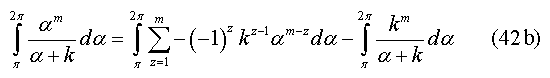
In this way the interval of q variation for one specific p is denoted by equation (50),
The figure 3, shows one graphical scheme of the q variation for one specific p; the dark line denotes the region in which the integral (here denoted by F(p,q)) has solution, which means for one specific p the integral F(p,q) is solved only in the region limited between q min and qmax.
ANALYSIS OF THE RESULTS
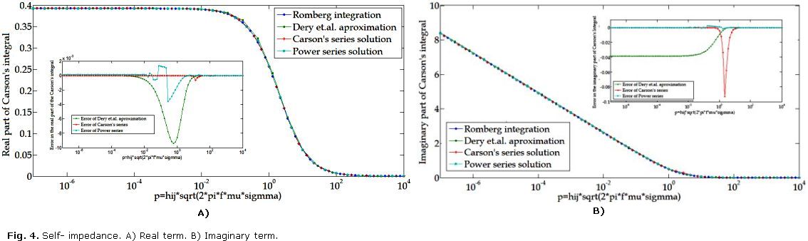
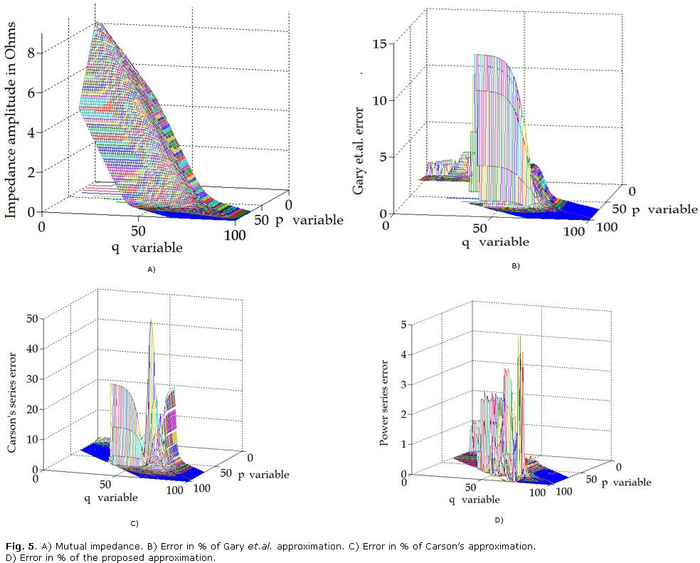
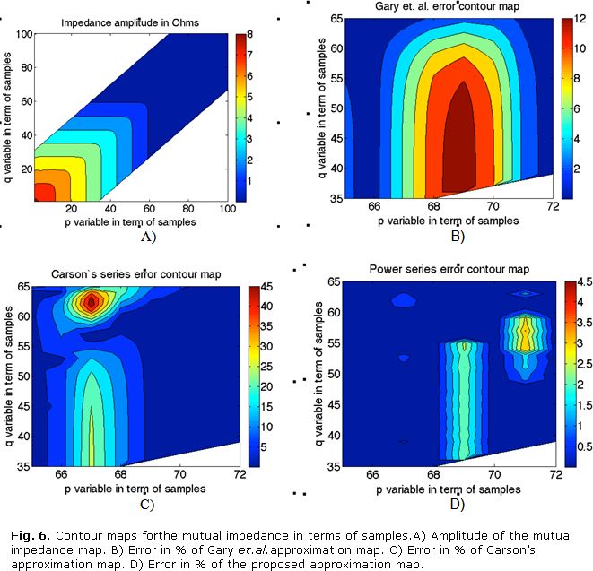
One has for the self-impedance p = hij(√ωμσ ) and q = 0 [3], so the self-impedance is function solely of p. While figure (4a), shows the results for the real part, figure (4b), shows the results for the imaginary one. Taking into account that the Carson's series solution is chosen like the best one (lower error) between the two Carson's proposed formulation. For both cases it is taken the Romberg integration results like a reference; means, the errors are referred to these results. For the mutual impedance one has p = (hi + hj)Φ and q = x with Φ = (√ωμσ) [3]. Figure 5, hows the obtained results taking the solution of the Romberg integral as a reference. Here, as for the self-impedance, it is taken the best Carson's solution, nevertheless there are big errors in some specific points in which no one of the Carson's series converge; for this reason it is necessary to know, previously to the use of Carson's series, if one is in the non-convergence zone. The variables p and q are discretized from the minimum to the maximum value taken 100 samples logarithmically spaced, for this reason in figures 5, and 6, p and q are in terms of number of samples. As it was showed in figure 3, there are some samples that not exist because q is function of p and for one specific p there are only some q's.
Figure 6, shows the contour maps for the mutual impedance in term of p and q samples. A figure 6a, show the points in which the impedance exists because corresponds to a logical p and q samples. Figures 6b, 6c and 6d, show the zone of maximum error for each approximation, this zone corresponds to the interval between samples 65-72 for p and 35 to 65 for q. The remaining impedances, for all cases, have lower errors, so it is not important to show them. Figure 6, shows the error distribution for all approximations; from this figure it's noticeable that there are no regions in which you obtain better solutions with Carson's series and/or Gary et.al. approximation than with the proposed solution. By the other hand, it is recommendable the use of simple formulas, as Gary et.al. ones in regions in which they have low error, and use the proposed solution in regions in which Gary et.al. approximation has not acceptable errors.
CONCLUSIONS
In this work it is developed a new solution for the Carson's integrals, the proposed solution is based on the definition of the upper limit of the integral, the power series expansion and the integral separation into some intervals. The new solution in comparison with the existing ones, taking the numerical solution like a reference, gives betters results; so, although its complexity this is a new and novelty analytical solution for the Carson's integrals and it is a really good option to obtain the ground impedance in region in which the existing solutions have not acceptable errors.
REFERENCES
1. WEDEPOHL, L.M.; WASLEY, R.G., "Wave propagation in multiconductor overhead lines calculation of series impedance for multilayer earth". Proceedings of the Institution of Electrical Engineers, IET, 1966, vol.113, n.4, p. 627-632, Disponible en: http://dx.doi.org/10.1049/piee.1966.0102, ISSN 0020-3270.
2. CARSON, J.R., "Wave propagation in overhead wires with ground return". Bell Systems Technology Journal, 1926, vol.5, n.4, p. 539-554, Disponible en: http://dx.doi.org/10.1002/j.1538-7305.1926.tb00122.x, ISSN 0005-8580.
3. DERI, A., "The complex ground return plane: A simplified model for homogeneous and multi-layer earth return". IEEE Transactions on Power Apparatus and Systems, IEEE, 1981, vol. PAS-100, n.8, p. 3686-3693, Disponible en: http://dx.doi.org/10.1109/TPAS.1981.317011, ISSN 0018-9510.
4. URIBE, F.A.; et al., "Ground-impedance graphic analysis through relative error images". IEEE Transactions on Power Delivery, IEEE, 2013, vol.28, n.2, p. 1235-1237, Disponible en: http://dx.doi.org/10.1109/TPWRD.2013.2248960, ISSN 0885-8977.
5. URIBE, F.A., "Ground-Wave Propagation Effects on Transmission Lines through Error Images". Ingeniería Investigación y Tecnología, 2014, vol.15, n.3, p. 457-468, [consultado: octubre de 2014], Disponible en: http://www.ingenieria.unam.mx/~revistafi/ejemplaresHTML/V15N3/V15N3_art11.php, ISSN 1405-7743.
6. IEEE Standard 356-2010, IEEE Guide for Measurements of Electromagnetic Properties of Earth Media. 2011, p. 1-63, Disponible en: http://dx.doi.org/10.1109/IEEESTD.2011.5742810, E-ISBN: 978-0-7381-6448-9.
7. IEEE P356/D8, July 2010, IEEE Draft Guide for Measurements of Electromagnetic Properties of Earth Media. 2010, p. 1-63, [consultado: agosto de 2014], Disponible en: http://www.ieeeexplore.com/servlet/opac?punumber=5511468, E-ISBN: 978-0-7381-6408-3.
8. COETZEE, P., "A technique to determine the electromagnetic properties of soil using moisture content". South Africa Journal of Science, 2014, vol.110, n.5-6, p. 1-4, [consultado: mayo de 2014], Disponible en: http://www.scielo.org.za/scielo.php?pid=S0038-23532014000300015&script=sci_arttext, ISSN 0038-2353.
9. LAI, W.L.; et al., "Frequency-dependent dispersion of high-frequency ground penetrating radar wave in concrete". NDT & E International, 2011, vol.44, n.3, p. 267-273, Disponible en: http://dx.doi.org/10.1016/j.ndteint.2010.12.004, ISSN 0963-8695.
10. ROSAS, G.; et al., "Efficient truncation criterion for the parameter estimation of a stratified ground block". IEEE Transactions on Power Delivery, 2013, vol.28, n.4, p. 2534-2535, Disponible en: http://dx.doi.org/10.1109/TPWRD.2013.2258819, ISSN 0885-8977.
11. URIBE, F.A., RAMIREZ, A., "Alternative series-based solution to approximate pollaczek's integral". IEEE Transactions on Power Delivery, 2012, vol.27, n.4, p. 2425-2427, Disponible en: http://dx.doi.org/10.1109/TPWRD.2012.2202199, ISSN 0885-8977.
12. URIBE, F.A., "Numerical Infinite Series Solution of the Ground-Return Pollaczek Integral". Ingeniería Investigación y Tecnología, 2015, vol.16, n.1, p. 49-58, [consultado: octubre de 2014], Disponible en: http://www.ingenieria.unam.mx/~revistafi/ejemplaresHTML/V16N1/V16N1_art05.php, ISSN 1405-7743.
Recibido: febrero de 2014
Aprobado: septiembre de 2014
José Alberto Gutiérrez Robles. He received his B.Eng. in Mechanical and Electrical Engineering and his M.Sc. degrees from CUCEI-Universidad de Guadalajara in 1993 and 1998, respectively. He received his Ph.D. degree from Cinvestav, Guadalajara Campus, Mexico, in 2002. He is currently a full professor at the Department of Mathematics, CUCEI, University of Guadalajara, and México. His research interests are in applied mathematics, Power System Electromagnetic Transients and Lightning Performance. e-mail: jose.gutierrez@cucei.udg.mx

