Artículos

FPGA design of a Time-Variant Coefficient Filter

Fidel Cruz Garrido¹ 
http://orcid.org/0000-0003-3101-4598

Jorge Torres Gómez² 
http://orcid.org/0000-0001-9523-048X

¹LACETEL, Cuba

²Department of Digital Signal Processing, Technische Universität Chemnitz, 09126 Chemnitz, Germany.

ABSTRACT

Currently, a variety of solutions of Linear Time-Variant Filters (LTV) are reported to apply on Software Defined Radio, Radar and Sensor Networks systems. In contrast to Linear Time-Invariant Filters (LTI), LTV filters exhibit better performance regarding constraints on time domain such as risetime and overshoot parameters. Despite they have been used for a variety of applications, they are unable to reach certain processing speeds. To achieve the processing of higher data rates binary signals, it is necessary to reduce risetime of output filters, which is accomplished by properly changing the characteristic frequency parameter just on the transient time period. This article is related to the implementation of an LTV digital lowpass filter, to process binary and multilevel signals. The LTV filter represents a novel proposal with considerably shorter risetime. Implementation on a Field-Programmable Gate Array (FPGA) is addressed and discussed by using Xilinx System Generator software on MatLab. Results exhibit proper performance when a lowpass Bessel LTV Filter is considered.

Keywords: Linear Time-Variant Filter; Risetime; FPGA

1.- INTRODUCTION

Filtering is essential to process communication signals to improve the quality of the signal of interest. Some major reasons to apply are the need to suppress noise and interference or to discriminate between multiplexed signals [¹]. To that end, Linear Time-Variant (LTV) filters are reported to apply in a variety of fields such as control systems [²], communications [³], signal processing, biomedical applications [⁴] and circuit modeling [⁵].

Nowadays, several applications requiring filtering operations demand high commutation speed [⁶], which represents a difficult task to achieve relaying on LTI filters. According to [⁷], lowpass filtering is characterized by long transient states which introduce distortion that affects the output filtered signal. Filtering operations are limited by LTI systems due to fixed parameters, which entails a relatively large risetime. To derive lower values of risetime, the output filter response is restricted by the uncertain principle. This principle establishes theoretical and practical limits to obtain shorter risetime values and simultaneously to reduce noise when filter parameters are constant in time [⁸]. To this end, LTV filters are designed to overcome these constraints.

LTV filters perform a variation of internal coefficient values to reduce risetime, then to decrement distortion of the output filtered signal. Several design approaches are based on $S$ or frequency planes, dynamic change of hardware elements and the definition of proper curves for the filter coefficient values.

Laplace characterization for LTV filters is exposed by [²]. In this paper, the applicability of Laplace transform techniques for LTV filters is demonstrated by developing frequency-domain models applied to basic network elements. This paper establishes main in-out relations over which common LTV filter designs are structured.

Some designs of filters with variable cutoff frequency are not addressed to reduce risetime but to provide several available cutoff frequencies in the same design. A design method for Variable Digital Filters (VDF) is reported in [³]. This method proposes a Finite Impulse Response (FIR) Variable Digital Filter (VDF) described by a piecewise high attenuation function on the stopband. Additionally, the report in [⁹] employs a single lowpass prototype filter to obtain variable lowpass, highpass, bandpass and bandstop frequency responses. These filters can modify frequency response on-the-fly and represents a low complexity alternative to the other similar design reported in [¹⁰].

LTV filters topic is presented by [¹¹] through the definition of Linear Periodic Time Variational (LPTV) filters. A linear filter can be called an LPTV filter of period $M$ , when the filter behavior exhibits periodicity of the same period $M$ . A special case is provided by linear time invariant (LTI) filters, which represents an LPTV FIR filter of period one. Each different implementation brings insight into a particular aspect of system parameters such as the coefficients in the case of [¹¹]. Provided that LPTV systems can be represented by a periodic switch of LTI systems, then a new architecture is proposed by [¹²] comprised of banks of LTI filters. This new architecture is also a solution to some energy issues caused by a non-optimal use of the multipliers. Although the LPTV approach has the common objective of the variable change frequency response of filters, none of these approaches are derived to reduce risetime parameter.

Commonly, LTV techniques derive reduction of risetime parameter by synchronously changing coefficients during the transient interval of the filter, i.e. damping factor [⁷] and instantaneous bandwidth [⁸]. This approach has been widely used in several designs by stable LTV multi-notch Infinite Impulse Response (IIR) filters [¹³], IIR multi-notch filters [⁴] and FIR [¹⁴] filters. Typically, instantaneous bandwidth changes according to a heuristic function of time. By these methods, a variety of simulation and obtained results confirmed the advantage over the stationary counterpart LTI filters in terms of reducing the transient period length.

Designing time-variant filters on Field Programmable Gate Array (FPGA) devices is recommendable due to inherent re-programmable characteristics from reconfigurable hardware. By means of FPGA devices, dynamic of parameters is commonly allowed to implement for filtering operations to further improve integration, processing speed and expanding system capabilities. Taking advantage of these features a variety of solutions are reported to devise digital signal processing methods on FPGA. For instance, some recent solutions are reported to FIR filter design by using Stratix II FPGA [¹⁵], self-programmable filter on Xilinx FPGA including Embedded Microprocessors [¹⁶], FIR filter design subject to energy constraints [¹⁷] and smooth filtering of multispectral satellite images [¹⁸] to improve quality.

Current work addresses the design of an LTV filter to implement on FPGA devices based on the report in [⁸], which is inspired in the widely consulted work presented in [¹⁹]. Then to carry out several simulations to validate performance. Based on the design exposed by [⁸] it is expected to preserve, on the proposed digital design, main time restrictions such as risetime and overshoot. The current article is organized as follows: Section 2 describes the digital design and filter implementation on FPGA, Section 3 discusses the main results and concluding remarks are presented in Section 4.

2.- DIGITAL DESIGN OF THE TIME VARIANT FILTER

Similar to LTI filters, the design of LTV filters demands to devise the transfer function, then to implement on a given technology. Current section analyses the reported LTV design of second- and fourth-order systems and the proposed implementation on FPGA.

2.1.- FILTER SPECIFICATIONS DESCRIPTION

Filter specifications are established by a second-order lowpass filter with cutoff frequency ${\omega }_c$ through Bessel approximation [¹²]. In this case, the following transfer function is employed:

$\mathrm{H}\left(\mathrm{s}\right)=\frac{1}{\frac{{\mathrm{s}}^2}{{\mathrm{\omega }}_0^2{\mathrm{\omega }}_{\mathrm{c}}^2}+\frac{2\mathrm{\beta }\mathrm{s}}{{\mathrm{\omega }}_0{\mathrm{\omega }}_{\mathrm{c}}}+1},$ (1)

where ${\text{ω}}_0{\omega }_c$ is the characteristic frequency, ${\text{ω}}_{\text{c}}$ is the cutoff frequency and $\text{β}$ is the damping factor. Thus far, the designed filter in (1) is similar to an LTI Filter. The LTV filter is extended from (1) by time-varying the coefficient ${\text{ω}}_0\left(t\right)$ along time. The variation of the coefficient ${\omega }_0\left(t\right)$ is repeatedly applied on each rising or falling edge of the received binary signal, as shown in Fig. 1. The sequence for the coefficient ${\omega }_0\left(t\right)$ depicted in Fig. 1b) is synchronized to rising and falling edges of the received signal in Fig. 1a).

Values for ${\omega }_0\left(t\right)$ are derived based on the solution of a variational problem subject to bandwidth restrictions as described in [⁸]. The condition that must satisfy ${\omega }_0\left(t\right)$ to optimally reduce the risetime at the filter output is given after solving:

$\frac{{\mathrm{t}}^2{\mathrm{e}}^{-\mathrm{\beta }{\mathrm{\omega }}_0\mathrm{t}}}{\sqrt{1-{\mathrm{\beta }}^2}}\mathrm{ }\mathrm{R}\cos \left(\mathrm{\theta }\right)+\mathrm{\lambda }=0,$ (2)

for ${\omega }_0$ , where $\text{t}$ represents time and ${\mathrm{R}}_{21}=\sqrt{{\mathrm{\omega }}_0^2{t}^2-2\beta {\mathrm{\omega }}_{0}t+1}$ , $\mathrm{\theta }={t\mathrm{\omega }}_0\sqrt{1-{\mathrm{\beta }}^2}-{\text{tan}}^{-1}\frac{1-\mathrm{\beta }{\mathrm{\omega }}_{0}t}{{t\mathrm{\omega }}_0\sqrt{1-{\mathrm{\beta }}^2}}$ , and $\mathrm{\lambda }={10}^{-12}$ . Solutions for ${\text{ω}}_0$ that satisfy relation in (2) are obtained by numerical methods. These curves are encountered by a combination of bisection, secant, and inverse quadratic interpolation methods when t is varied from $0$ to $6·{10}^{-4}$ in steps of ${10}^{-6}$ seconds as determined in [⁸].

Figure 1 Binary input signal. b) Characteristic frequency of second-order systems. 

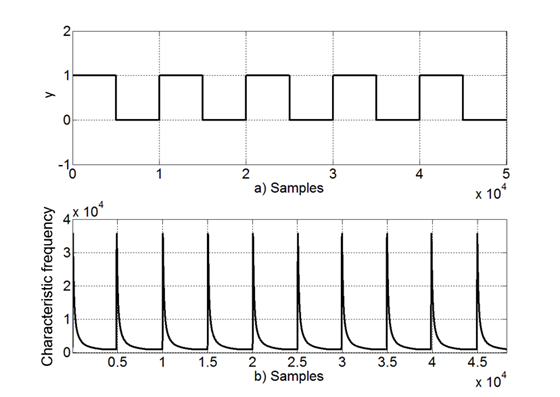
The solution to the optimization problem, provided after solving (2), optimally reduce the risetime parameter of the filter output. The sequence for ${\omega }_0\left(t\right)$ , as depicted in Fig. 1b), performs an increment of the instantaneous bandwidth of the filter when rising or falling edges are received on the incoming signal. This is in accordance with the higher values of instantaneous bandwidth around rising and falling edges. Hence, from a qualitative standpoint, this approach decrements risetime parameter of the output filtered signals.

In practice, to device the second-order system from (1) with the time-varying coefficient ${\omega }_0\left(t\right)$ , it is needed to implement a state-variable diagram as depicted in Fig. 2. This diagram consists of a second-order loop through the cascade of two integrator blocks where the ${\omega }_{0i}\left(t\right)$ represents the varying coefficient ${\omega }_0\left(t\right)$ [²²].

Figure 2 State-variable diagram for second-order System. 

Although the LTV system in (1) with a time-varying coefficient ${\omega }_0$ represents a second-order system, higher-order systems may be devised by concatenating similar systems. For instance, after connecting in cascade two similar systems to (1), then the following fourth-order system is derived [⁸]:

$\mathrm{H}\left(\mathrm{s}\right)=\frac{1}{\frac{{\mathrm{s}}^2}{{\mathrm{\omega }}_{01}^2{\mathrm{\omega }}_{\mathrm{c}}^2}+\frac{2{\mathrm{\beta }}_1\mathrm{s}}{{\mathrm{\omega }}_{01}{\mathrm{\omega }}_{\mathrm{c}}}+1}\bullet \frac{1}{\frac{{\mathrm{s}}^2}{{\mathrm{\omega }}_{02}^2{\mathrm{\omega }}_{\mathrm{c}}^2}+\frac{2{\mathrm{\beta }}_2\mathrm{s}}{{\mathrm{\omega }}_{02}{\mathrm{\omega }}_{\mathrm{c}}}+1},$ (3)

where values of ${\text{ω}}_{\text{c}}$ , ${\text{ω}}_{01}$ , ${\text{ω}}_{02}$ , ${\text{β}}_1$ , ${\text{β}}_2$ have a similar meaning to the system in (1). The current article addresses the implementation of a fourth-order LTV filter on FPGA. This procedure may be extended to higher-order systems by concatenating additional transfer functions of first and second orders then to derive proper values of ${\text{β}}_i$ and ${\text{ω}}_{0\text{i}}$ as described in [⁸].

2.2.- FILTER IMPLEMENTATION ON FPGA

Current Section proposes the functional implementation on FPGA of a discrete version of the system in Fig. 2, but concatenated in cascade to have a fourth-order system. To this end, blocks of Simulink Xilinx Blockset are employed relaying on System Generator Software (SYSGEN) 12.4. Similar filter designs may be afforded by using this configuration. Fig. 3 exhibits the general scheme to process the input signal, corresponding to that described in [¹⁹].

Two main blocks are connected, the Coefficients Update block to conform the time-varying filter coefficients ${\text{ω}}_{01}$ , ${\text{ω}}_{02}$ , and the LTV Filter block to process the input signal. Blocks beta1 and beta2 store the values for constants ${\text{β}}_1$ and ${\text{β}}_2$ , which are approximately equal to $0.958$ and $0.621$ , respectively.

Figure 3 General Scheme of the Filter with Time-Varying Parameters. 

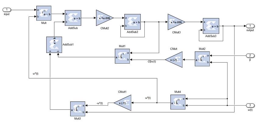
LTV Filter block is implemented by two identical second-order systems. Fig. 4 depicts the obtaining of one of the second-order systems from the LTV Filter block in Fig. 3. Both of them are structurally identical and are connected in cascade as depicted in Fig. 5, only the coefficient values are different. The implementation of the second-order system in Fig. 4 is a direct discrete representation of the state-variable diagram in Fig. 2. The integrators are implemented by the transfer function $\frac{1}{1-z^{-1}}$ (impulse invariance method [²³]), multipliers and adders are implemented by the counterpart FPGA blocks. Elements are connected in analogy to the state block diagram in Fig. 2.

Figure 4 First Section of the Fourth-Order IIR filter. 

Figure 5 Two-Sections Preprocessing Filter. 

Coefficient Update block provides the time-varying coefficient sequences ${\text{ω}}_{01}$ and ${\text{ω}}_{02}$ . Both sequences must be synchronously restarted to falling and rising edges of the received signal as depicted in Fig. 1 b). In this regard, the system depicted in Fig. 6 attempts to detect edges on the input signal by the Preprocessing and Detection blocks, then to restart the Coefficients Storage block to output the sequence of the proper coefficients. The preprocessing subsystem reduces the unwanted effect of noise for the next subsystems.

Figure 6 General Scheme of the Coefficient-Updating System. 

The Preprocessing block in Fig. 6 is implemented by using a third-order IIR lowpass filter. The normalized cutoff frequency is equal to the number of samples in a semi period of the binary input signal. This value reduces as much as possible undesirable input noise and preserves main frequency components of the binary signal simultaneously. The coefficients of the IIR lowpass, of the Preprocessing block, were derived by using the software fdatool of Matlab. The filter was implemented by using Direct Form II method as depicted in Fig. 7 [²³]. Direct Form II is selected due to the reduction on the total numbers of delay elements. Filter coefficients were exported from fdatool and obtained the structure shown in Fig. 7.

Figure 7 Scheme of First Section of the Preprocessing Filter. 

Following the Preprocessing subsystem, the Detection subsystem is implemented as depicted in Fig. 8. To detect when the input signal in “In” intersects the threshold value in “Threshold” a comparator is used by the Relational block. The threshold value is established on $0.5$ assuming a normalized input signal. The output of the Relational block is then differentiated to itself by a delayed version using de Delay and Logical blocks. This produces levels in 1 on instants when the input signal “In” reaches the input signal “Threshold”.

Figure 8 Scheme of the Detection Subsystem. 

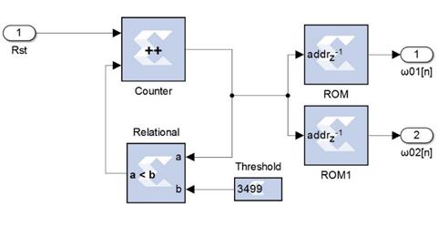
The Coefficients Storage subsystem is implemented as depicted in Fig. 9. Time-varying coefficients are stored on ROM blocks and these are continuously fetched by the Counter block. The Counter block output values ranged from zero to the length of the ROM stored sequence. In case that the counter output value reaches the length of ROM stored sequence, then the counter is disabled by the Relational block. This is needed to avoid overflow to access ROM blocks.

Figure 9 Scheme of the Coefficients-Storage Subsystem. 

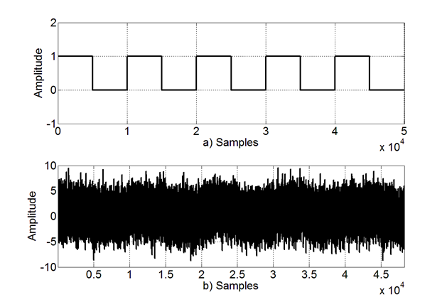
To illustrate the overall functionality of the system in Fig. 6, Fig.10 exhibits signals from the Scope block by Signals A, B, C and D. Based on the noisy binary signal in Fig. 10 a) (Signal A), the preprocessing block reduces noise at the output in Fig. 10 b) (Signal B) by IIR filtering input samples. This is needed to cancel out noise and better detect binary transitions on the received signal. Based on the Preprocessing output Signal B, the detection block outputs ones on the binary transitions of the received signal, this is depicted in Fig. 10 c) (Signal C). Then, Signal C restarts the Coefficients Storage Block to produce Signal D, where the values of the coefficients are restarted on each input signal transition. Fig. 10 d) represents the final output of the system in Fig. 6.

3.- RESULTS

To derive results of the implemented scheme in Fig. 3, main parameters of filter specifications were settled as follows: ${\beta }_{01}=0.958$ , ${\beta }_{02}=0.621$ and ${\omega }_c=1000 rad/s$ . Elements on the FPGA are implemented by using an arithmetic precision of 32 total bits and 16 bits to have the binary point representation. Fig. 11 a) represents the rectangular pulse train used to each simulation. In this case, the income signal is of unit amplitude and 5000 samples on each level length. Transmitted signal to be recovered was conducted through a channel modeled by Additive White Gaussian Noise (AWGN). This conforms the received contaminated signal to be processed by the LTV filter. This is depicted in Fig. 11b).

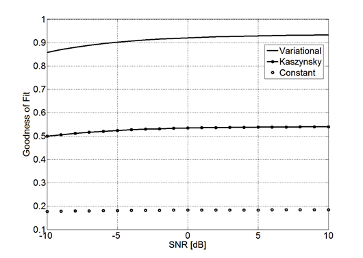
Fig. 12 exhibits results of the implemented system for a variety of design: constant coefficients (LTI), Kaszynsky [⁷] and the Variational method reported in [⁸] when Signal to Noise Ratio (SNR) parameter equals to $-10$ dB. These designs represent main solutions for LTV IIR filtering. LTV filters (Kaszynsky and Variational) reduce dramatically the risetime parameter in comparison to LTI filters. These results are similar to report in [⁸] which in turn establishes proper performance of the proposed FPGA design.

To measure the quality of filtered signal, Goodness of Fit tests were evaluated. This is calculated using a cost function given by the Normalized mean square error [²¹]:

$\mathrm{ }\mathrm{ }\mathrm{G}\mathrm{o}\mathrm{F}=1-\sum _{n=1}^{n=N}{\left(\frac{x\left[n\right]-x_{ref}\left[n\right]}{x\left[n\right]-{\stackrel{-}{x}}_{ref}}\right)}^2,\mathrm{ }$ (5)

Where $N$ is the total number of samples, $x\left[n\right]$ and $x_{ref}\left[n\right]$ are the nth-sample value of the filtered signal and the reference signal, respectively. Value of ${\overline{x}}_{ref}$ is the mean value of the filtered signal.

The metric in (5) was used to establish a comparison between the ideal input signal represented in Fig. 11 a), and the output filtered signal on the SNR range $[-10 10]$ . The closer the value of (5) to one, the more alike are the filtered and the transmitted signal. The test was made for the Constant Parameter, the Kaszynsky, and the Variational method. The results are depicted in Fig. 13. Each curve in Fig. 13 exhibits a monotone relation between Goodness of Fit and SNR parameter. Despite the Kaszynsky Filter is better than the constant LTI, the Variational filter has the best performance provided the Goodness of Fit is near to unity.

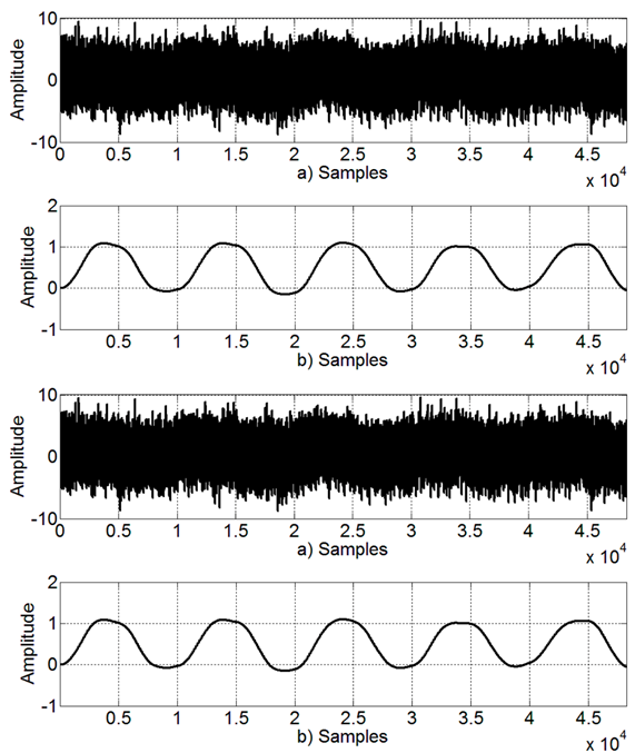
Figure 10 Detection block performance a) Input of Preprocessing block. b) Output of Preprocessing block. c) Output of Detection block. d) Characteristic frequency.  

Figure 11 Bipolar signal without noise. b) Input of Preprocessing Subsystem. 

Figure 12 Filtered Output Signal. 

Figure 13 Goodness of Fit vs. SNR curves. 

A quick resource estimation needed to build this filter is shown in Table 1. The total number of components is lower than commonly available resources on FPGAs. For instance, on a Spartan3 board with a XC3S500E FPGA device, the occupation percentage of the DSP48A1s is 82%, 22% of the Slices and 52% of the RAMB16BWERs. These occupancy values on FPGA indicate an affordable solution to implement. However, it may be needed an FPGA device with increased features for more complex applications that require the addition of additional intellectual property modules.

4.- CONCLUSIONS

Many modern applications of filters demand the processing of high data rate signals. Under these conditions, it is essential to reduce risetime parameter of filters as much as possible. LTI filters are limited by the constant bandwidth to process signals of shorter time symbol duration. However, LTV filters are reported to circumvent this problem by time-varying coefficients. A design for FPGA implementation of a time-varying parameters filter has been presented in this work. In this case, a fourth-order lowpass filter was designed by Bessel approximant function and using Xilinx System Generator (SYSGEN) software. The proposed design is envisaged to further employ FPGAs capabilities to dynamically reconfigure main parameters. Simulations validated proper performance to reduce risetime parameter and improve the quality of received signal simultaneously. This reduction of risetime parameter allows filtering signals of higher data rates to increase the communication speed. Future work is pointed out to implement an odd filter order and to analyze energy restriction on the proposed design.

REFERENCES

1. F. S. Rocha, V. H. M. Biajo, H. de O. Mota, C. A. Maia, and F. H. Vasconcelos. Design and analysis of analog filters by statistical methods. 2018 IEEE International Instrumentation and Measurement Technology Conference (I2MTC); 2018.p. 1-6.

2. S. Erfani, M. Ahmadi, and N. Bayan, "Signal analysis in linear time-varying systems. 2013 International Symposium on Signals, Circuits and Systems (ISSCS); 2013.p. 1-4.

3. T. Miyata and N. Aikawa. A design method for complex coefficient FIR filters with variable stopband characteristics. Communications and Signal Processing (ICICS) 2013 9th International Conference on Information; 2013.p. 1-5.

4. S. Kocon and J. Piskorowski. Time-varying IIR multi-notch filter based on all-pass filter prototype. Methods and Models in Automation and Robotics (MMAR), 2014 19th International Conference On; 2014.p. 112-118.

5. A. Ambede, S. Shreejith, A. P. Vinod, and S. A. Fahmy. Design and Realization of Variable Digital Filters for Software-Defined Radio Channelizers Using an Improved Coefficient Decimation Method. IEEE Trans. Circuits Syst. II Express Briefs; 2016;63(1): 59-63.

6. A. Ambede and A. P. Vinod. Design and Implementation of High-Speed All-Pass Transformation-Based Variable Digital Filters by Breaking the Dependence of Operating Frequency on Filter Order. IEEE Trans. Very Large Scale Integr. VLSI Syst.; 2016;24(5): 2008-2012.

7. R. Kaszynski. A proposal of non-stationary low-pass Chebyshev's filters. 1996 IEEE Conference on Emerging Technologies and Factory Automation, 1996. EFTA '96. Proceedings; 1996.p. 759-762.

8. K. T. de la Garza, J. T. Gómez, R. C. de Lamare, and M. J. F.-G. García. A Variational Approach for Designing Infinite Impulse Response Filters With Time-Varying Parameters. IEEE Trans. Circuits Syst. Regul. Pap.; 2018; 65(4): 1303-1313.

9. A. Ambede and A. P. Vinod. Design of low complexity variable digital filters using first order all pass transformation and improved coefficient decimation method. 2014 2nd International Conference on Devices, Circuits and Systems (ICDCS); 2014.p. 1-5.

10. K. K. Prasad and C. Annadurai. Reconfigurable and low complexity variable digital filter design. 2014 International Conference on Communications and Signal Processing (ICCSP); 2014.p. 1260-1263.

11. S. S, R. Dhuli, S. K, and L. H. V. P. Puvvada. Low complexity architecture of linear periodically time varying filter based on a switching representation. 2013 National Conference on Communications (NCC); 2013.p. 1-5.

12. D. Niranjan and B. Ashwini. Noise cancellation in musical signals using adaptive filtering algorithms. 2017 International Conference on Innovative Mechanisms for Industry Applications (ICIMIA); 2017. p. 82-86.

13. P. Okoniewski, S. Kocon, and J. Piskorowski. Design of stable LTV multi-notch IIR filter with Lookup Tables. 2017 22nd International Conference on Methods and Models in Automation and Robotics (MMAR); 2017. p. 248-252.

14. S. Kocon and J. Piskorowski. Time-varying FIR notch filter implementation using Raspberry Pi. 2015 20th International Conference on Methods and Models in Automation and Robotics (MMAR); 2015.p. 169-174.

15. J. Zheng and Z. Wei. FIR Filter Design Based on FPGA. in 2018 10th International Conference on Measuring Technology and Mechatronics Automation (ICMTMA); 2018.p. 36-40.

16. W. Hu, G. Zhang, and W. Li. Self-Programmable Multipurpose Digital Filter Design Based on FPGA. 2011 International Conference on Internet Technology and Applications (iTAP); 2011.p. 1-5.

17. Y. F. Kula, T. Ayhan, and M. Altun. Approximate implementation of FIR filters on FPGA. 2018 26th Signal Processing and Communications Applications Conference (SIU); 2018.p. 1-4.

18. P. S. Shakila, V. V. Thyagarajan, and S. Rajaram. FPGA implementation of filtering algorithm for multispectral satellite image. 2018 2nd International Conference on Inventive Systems and Control (ICISC); 2018.p. 1006-1010.

19. R. Kaszynski and J. Piskorowski. Selected Structures of Filters With Time-Varying Parameters. IEEE Trans. Instrum. Meas.; 2007; 56(6): 2338-2345.

20. L. A. Zadeh. Frequency Analysis of Variable Networks. Proc. IRE; 38(3):291-299.

21. MathWorks [serial en Internet]. MathWorks - Makers of MATLAB and Simulink. [Accessed: 13-Sep-2018]. Disponible en: https://www.mathworks.com/

22. D'Angelo H. Linear Time-Varying Systems: Analysis and Synthesis. Boston, MA: USA: Allyn & Bacon; 1970.

23. Oppenheim AV, Schafer RW. Discrete-Time Signal Processing: Pearson New International Edition. 3 ed. Harlow: Pearson Education Limited; 2013. 1056 p.

Received: September 17, 2019; Accepted: March 10, 2020

CONFLICT OF INTEREST: There isn’t conflict of interest with the authors or any institution which they are affiliated with nor any other institution. The opinions that were expressed here are only responsibility of the authors and don’t represent the stand of the institutions which they are affiliated with.

AUTHORS’ CONTRIBUTION: Both authors contributed equally to the realization of this article.

Fidel Cruz Garrido: BSc in Telecommunications and Electronics. E-mail: [e-mail]; [e-mail] ORCID: 0000-0003-3101-4598Affiliation: Department of I+D+i, LACETEL, Cuba. His researching interests include digital signal processing, cognitive radio systems, power line communications and microprocessors programming.

Jorge Torres Gómez: BSc in Telecommunications and Electronics, MSc and PhD in Telecommunication Systems. E-mail: [e-mail]; [e-mail] ORCID: 0000-0001-9523-048X. Affiliation: Department of Digital Signal Processing, Technische Universität Chemnitz, 09126 Chemnitz, Germany. His research interests include digital signal processing, cognitive radio networks and software-defined radio.