Artículo de investigación científica y tecnológica

Methodology for the preparation and selection of black box mathematical models for the energy simulation of screw type chillers

Metodología para la confección y selección de modelos matemáticos de caja negra para la simulación energética de enfriadoras tipo tornillo

Yamilé Díaz-Torres^{I  *} 
http://orcid.org/0000-0002-8729-7032

Miguel Santana-Justiz^I 
http://orcid.org/0000-0003-3586-8515

Gilberto Jose Francisco-Pedro^II 
http://orcid.org/0000-0003-0490-1781

Lazaro Daniel-Alvarez^III 
http://orcid.org/0000-0003-0948-1632

Yudit Miranda-Torres^I 
http://orcid.org/0000-0001-9799-1186

Mario Álvarez Guerra-Plascencia^I 

^IUniversidad Carlos Rafael Rodríguez, Facultad de Ingeniería. Cienfuegos, Cuba

^IIInstituto Médio Politécnico do Namibe Número:55 Pascual Luvualu. Angola

^IIIEmpresa de Farmacias y Opticas. Cienfuegos,Cuba

ABSTRACT

This article proposes a methodology for the construction and simultaneous evaluation of black box models for screw type water chillers. The estimation method used was generalized Least Squares. The proposed methodology is an iterative process and its evaluation is based on quality parameters of goodness of fit and statistical assumptions. Ten mathematical models with different levels of complexity were proposed. The statistical software used was Eviews 7.0. The selection of the models was based on the Occam's razor, remaining as the most feasible model is model 5 characterized by a multiple linear regression

Key words: chiller; black box models; linear regression

RESUMEN

El presente artículo propone una metodología para la construcción y evaluación simultánea de modelos de caja negra para enfriadoras de agua tipo tornillo, empleando el método generalizado de los mínimos cuadrados. La metodología propuesta es un proceso iterativo y su evaluación se basa en parámetros de calidad de la bondad del ajuste y los supuestos estadísticos. Se propusieron 10 modelos matemáticos con distintos niveles de complejidad. La comprobación de los modelos se efectuó empleando el programa estadístico Eview-7.0 la selección de los modelos se basó en el principio de la navaja Ockham, quedando como el modelo más factible es el modelo 5 caracterizado por un modelo de regresión lineal múltiple.

Palabras clave: enfriadoras de agua helada; modelos matemáticos de caja negra; regresión lineal

INTRODUCTION

The modelling of a centralized chiller system is the essential axis for the problems solution of optimization, design, diagnosis or prognosis of failures of these systems. Simulation involves developing mathematical models of the different sub-components (for example, the chiller, the pumping system, the condensation system, etc.). In addition, link it with the thermal dynamics of the building and the boundary conditions where the system develops, obtaining as a result the behaviour and/or prediction of energy parameters, system efficiency or possible thermodynamic states. To analyse a system in general, each of its sub-components can be considered a system in itself. The mathematical models of them are derived from the physical laws that govern the processes that take place and the state of the working substances inside and outside the limits of their operation.

To determine in real time, the energy consumption of a chiller, three types of mathematical models can be used: white box models, black box models and gray box models. Due to their relative simplicity and ease to obtain it, black box models are the most useful in engineering. These are empirical models that only depend on the operation parameters of a chiller. Manufacturer data or measurements are required, both must include a wide range of operating conditions for these machines [¹]. The black box model numerically relates the results or outputs with the most influential inputs. Its restriction is given in that it does not allow interpolating data that is outside the range so it cannot reflect the effects of any factors whose influence was omitted in its derivation. Their results also do not explain in detail the physical phenomenon that technology incurs. [²]

Black box models can be built in various ways. For example, [¹,³-⁹] used multiple linear regression. Other studies conducted by [¹⁰] used the Cox regression model. Le Cam [¹¹] used the kernel regression technique. Nowadays, artificial intelligence is frequently used to make these models, such as Neural Networks, for example the studies presented by Kusiak [¹²], Wei [¹³] and Jia [¹⁴], the Genetic Algorithm, presented by Wang [¹⁵] and neuro-fuzzy models through the study published by Atta [¹⁶]. Other published research used more complex methodologies for the preparation of these models such as self-regressive movement models [¹⁷]. Jenkins box models [¹⁷]. Support machines least squares vector for regression [^{18, 19}]; among others.

In the black box model specifically applied to the chiller, the dependent or output variable is established depending on the objective of the study. For example, the Operating Coefficient (COP), [⁶, ²⁰]; The electrical power consumed by the compressor [⁵, ⁸, ⁹]. The rated cold power or cooling capacity, [⁴, ⁹]. Cold water outlet temperature or set point temperature [¹⁷], among others. Likewise, the independent or predictive variables can be diverse, they can be used individually or in combination. For example, Wei [¹³] determined electric energy consumption through the variables: mass flow of ice water, in and out temperature difference of the condenser and air enthalpy. The model constructed by Yan et al. [²¹] used the partial load coefficient or load ratio (PLR) and the water temperature at the condenser inlet. Browne [²²] and Cheng [²³] also added the set point temperature. Qiu [²⁴] replaced the PLR with the cooling capacity. Other predictive variables that have been used in the construction of the model are: The compressor speed used by Romero [¹⁷], Le Cam [¹¹] employs climatological variables as outdoor temperature and relative humidity and more specific information has also been used as hours/day. Both dependent and independent variables are derived in a curve, which employ a series of parameters or correlation coefficients that allow their adjustment.

In the literature, methodologies for the construction and validation of models have been presented, for example, ASHRAE Guide 14 [²⁵] displays a guide to develop regression models for buildings, as well as a set of statistical metrics to assess the quality of construction. Model. Wang [²] presented a methodology to evaluate the energy consumption of centrifugal chiller. Gunay [²⁶] used the correlation matrix to assess the non-collinearity of the various variables that affect the functioning of the chillers. On the other hand, it is usual to present only a regression model and show only values of statistical indicators such as the correlation coefficient [R2], RMSE, coefficient of residuals variation, among others. However, in general, there are few articles that deal with the selection and validation of statistical models, the formalities that are required, or simply show the step by step for obtaining and selecting the regression model. The following article shows a methodology for the preparation and selection of mathematical models using the least square method.

METHODS AND MATERIALS

Methodology for the construction of black box type mathematical models for chillers

The model complexity level, the total predictor variables and regression coefficients, will depend on the data, as well as the results of the fit quality tests. According to Gunay [²⁶], a consensus must be reached between the number of dependent variables and the correlation coefficients, in order to avoid failures or adjustments to the black box model. Figure 1 shows the heuristic iterative methodology for the preparation and selection of several mathematical models of the selected chillers.

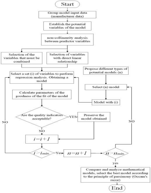
Source: own elaboration

Fig. 1 Heuristic methodology for the construction and selection of mathematical black box models.  

The methodology presented in figure 1 considers two explanatory variables. Expression 1 describes a multiple linear regression model, where Y is the response vector, X is the matrix of the explanatory or return variables, β represents the vector of the regression coefficients and ϵ is the model error as can see in expression 1

$\text{Y=}\beta \text{X+}\in$ (1)

This model is adjusted or not by calculating the estimators of the model parameters using the least squares method. The development of a regression model is based on a group of statistical assumptions, most of them in relation to the disturbance term. These are expression 2 and 3

a) Stochastic disturbances

$ui(i=\mathrm{1,......,}n)$ (2)

The mean is equal to zero

$\text{E(}ui\text{)}=\text{0}$ (3)

b) Homocedasticity. Stochastic disturbances are show in expression 4-9

$u_i(i=\mathrm{1,......,}n)$ (4)

They have the same variance.

$V(u_i)=E{\left[u_i-E(u_i)\right]}^2=E(u_i^2)={\sigma }_u^2$ (5)

Annotation

$V(u_i)={\sigma }_u^2$ (6)

Indicates that the variance does not change with the index i. Failure to comply of this assumption is called heterocedasticity.

$V(u_i)={\sigma }_u^2$ (7)

Although many statistical tests have been developed to verify the presence of homocedasticity in the regression models, it cannot be said that there is a definitive or always useful one. For this case, the White test [²⁷] is applied. This is one of the most robust tests because it is not based on any assumption about the nature of heterocedasticity. The white test approach is as follows:

$H_0:{\sigma }_i^2={\sigma }^{2}foralli.otherwise{H}_1:itisnotverifiedi.$ (8)

The realization of this contrast is based on the regression of the least squared errors, which are perturbations variance indicative, compared to an independent term, the regressors, their squares and their crossed products two to two. Thus, the auxiliary regression that allows the realization of this contrast is as follows:

$e_i^2={\delta }_0+{\delta }_{1}DI{F}_{t-1i}+{\delta }_{2}R{P}_{ti}+{\delta }_{11}DI{F}_{t-1i}^2+{\delta }_{22}R{P}_{1i}^2+{\delta }_{12}DI{F}_{t-1i}R{P}_{ti}+vi\begin{array}{cc}& i=\mathrm{1,...,}N\end{array}$ (9)

The statistic proposed for the realization of this contrast is λ = NR², where R² is the determination coefficient of the auxiliary regression. Under the null hypothesis, this statistic is distributed asymptotically as a ²(p), where p is the number of variables included in the auxiliary regression, except for the independent term. If the sample value of the statistic is high enough that the probability of rejecting the null hypothesis being true is less than 1%, we will reject the null hypothesis of homocedasticity

c) The absence of autocorrelation or serial correlation. Stochastic disturbances are mutually orthogonal $u_i$ and, $u_j$ they have zero covariance. This assumption its reflects in expression 10:

$Cov(u_i,u_j)E\left\{\left[ui-E(ui)\right]\left[u_j-E(u_j)\right]\right\}=E(u_i{u}_j)=0\forall i\ne j$ (10)

Failure to comply of this assumption is called autocorrelation, covariance $E(u_i{u}_j)\ne 0$ for some $i\ne j$ . Some of the factors that frequently involve the presence of autocorrelation in a model are: the exclusion of the variables model that are necessary; the inadequate specification of the functional model form; the delays inclusion of the explanatory variables in the model (distributed delay models), the inclusion of the dependent variable in a delayed form as an explanatory variable (autoregressive models), the existence of cycles and trend in the series, measurement errors , the previous manipulation of the data, the spatial proximity, in some series of cross-sectional data. To analyze the existence of self-correlation in a series. To verify the absence of autocorrelation in the residues of this model we will use the Breusch-Godfrey test [²⁸]. It is an autocorrelation test on errors and statistical residuals in a regression model. It makes use of the errors generated in the regression model and a hypothesis test derived from it. The null hypothesis is that there is no serial correlation of any order of ρ. The test is more general than that of Durbin-Watson, which is only valid for non-stochastic regressors and to test the possibility of a first-order autoregressive model for regression errors. The Breusch-Godfrey test has no restrictions, and is statistically more powerful than the statistic d. The steps to be performed in the contrast are: first, estimate the original model and obtain the series of estimated residues. Second, estimate the auxiliary regression equation with the expression 11:

${\widehat{e}}_t=\alpha +{\omega }_1{x}_1+{\omega }_2{x}_2+\dots +{\omega }_k{x}_k+{\delta }_1{\widehat{e}}_{t-1}+\dots +{\delta }_p{\widehat{e}}_{t-p}+{\in }_t$ (11)

Finally, when increasing the sample size, the product (np) R², where n is the number of observations, p the number of error delays used in the auxiliary regression and R² the coefficient of determination, follows a Chi-square distribution with p degrees of freedom. The hypothesis of self-correlation will be accepted when the value of the statistician exceeds the critical value of the Chi-square distribution at the level of statistical significance set

d) Normality.

Stochastic disturbances, see expression 12:

$u_i(i=\mathrm{1,......,}n)$ (12)

Have a normal distribution as show expression 13:

$u_i\text{~}N(\mathrm{0,}{\sigma }_u^2)$ (13)

This assumption does not directly influence the properties of the estimators, but is required to develop the inference methods used in the validation of the model. Thus, the violation of the assumption causes the F and t tests and the confidence intervals to lose reliability. To analyze the normality of a variable, the Jarque - Bera [²⁹], test will be used relatively simple and with direct implementation in the E-Views. The hypotheses of the Jarque Bera test [²⁹], its shows in expression 14:

$H_{\text{0}}\text{:u~}N{H}_{\text{0}}\text{:u}\ne N$ (14)

The test statistician is defined in the expression 15:

$JB=\frac{n-p}{6}\left[s^2+\frac{{\left(k-3\right)}^2}{4}\right]$ (15)

This statistician is distributed under the null hypothesis according to a chi-square distribution with two degrees of freedom. In its calculation p is the amount of estimated parameters, S is the so-called symmetry coefficient, measure, the symmetry degree of the distribution and K is the aiming point Kurtosis coefficient, the elevation of the distribution and the critical region takes the shape of the expression 16:

$W=\left\{JB:JB>X_{1-\alpha \left(2\right)}^2\right\}$ (16)

It should be taken into account, that if the available sample size is large enough, compliance with this assumption is no longer important.

Fulfillment of the classical assumptions for a regression model guarantees, in particular, that the estimators obtained by the least squares method are unbiased, consistent and efficient. At the same time, its non-fulfillment can invalidate many of the results that may be derived from the analysis of the model, or even the totality of said analysis, that is why the verification of fulfillment of the assumptions is an important part of the study.

Selection criteria to assess the ability to adjust models

Once an estimated equation has been obtained, it is necessary to evaluate in some way how well the estimates that it produces are adjusted to the corresponding observations of the dependent variable. For this, different measures or statisticians have been created whose current denomination is that of fit goodness measures, which is justified by the purpose for which they are intended.

• Determination coefficient (R²). It measures the variability proportion of the dependent variable Y , that is explained by the regression model, so that , it is used as a fit goodness measure. This value is obtained from the error squares sum (SSE) and of squares total sum (SST), from the expression 17:

$R^2=\frac{SSE}{SST}\begin{array}{ccc}& ,& 0\le R^2\le 1\end{array}$ (17)

The SSE corresponds to the distances squares sum of the points from the best fit curve determined by non-linear regression, while the SST is the distances squares sum of the points from a horizontal line corresponding to the measure of all the (Y) values without considering the effect of the explanatory variables (X). This determination coefficient fulfills with the property of always being a number between zero and one.

• Akaike information criterion (AIC) [³⁰]. The Akaike information criterion is a fit goodness measure of a statistical model. It can be said that it describes the relationship between bias and variance in the construction of the model, or generally speaking, about the accuracy and complexity of the model. The AIC is not a model test in the sense of hypothesis testing. Rather, it provides a means for comparison between models of a tool for model selection. Given a set of data, several candidate models can be classified according to their AIC. The model that has the minimum AIC is the best. From the AIC values, it can also be inferred that, for example, the first two models are more or less tied and the rest are much worse. In general, the AIC is defined as can see in expression 18:

$\text{AIC}=\text{2k-2*ln(L)}$ (18)

Where $\text{:k}$ It is the number of model parameters, and $\ln \left(L\right)$ It is the log-likelihood function for the statistical model. For smaller data sets, the $AI{C}_c$ second order correction applies, this it shows in expression 19:

${\text{AIC}}_{\text{c}}=\text{2*AIC}+\frac{\text{2k(k}+\text{1)}}{\text{N-k-1}}=\frac{2*N*k}{N-k-1}-2*\ln (L)$ (19)

Where, (N) is the size of the data sample. When the values of (AIC) are very close, the selection of the best model can be made based on the calculation of the probability, known as akaike weights, and the relative probability, evidence relationship, through the expression 20:

$probability={\text{e}}^{\text{-0}\text{,5}\Delta }/1+e^{-\mathrm{0,5}\Delta },\begin{array}{cc}relative& probability\end{array}=\frac{1}{e^{-0.5\Delta }}$ (20)

Where (Δ) is the difference between the AIC values

• Root Mean Squared Error (RMSE). The RMSE is a measure that groups the variability of those factors that the researcher does not take into account. The variance of (n) residuals ( $e_i$ ) is represented in expression 21:

$RMSE=\frac{{\displaystyle \sum {\left(e_i-\overline{e}\right)}^2}}{n-K}=\frac{{\displaystyle \sum e_i{}^2}}{n-K}=\frac{SCE}{n-K}$ (21)

Where, $\overline{e }$ is the measure of n residuals that in all cases correspond to zero, (K) is the number of parameters estimated in the model and (SSE) is the vertical distances squares sum of the points from the regression curve (residual). Once the (RMSE) corresponds to the residual variance, the models selected for their greater adjustment capacity are those that express the lowest value in that criterion.

Finally, after selecting several models and the results, the model that meets the quality assumptions and presents a high level of correlation will be selected; the final choice will depend on the principle of parsimony that establishes that from the considered models the simplest must be chosen.

Black box model for a air-cooled screw water chiller

For the construction of the mathematical models, it is required to use operating data of the selected chillers. These can be real data of the machine exploitation or in the absence of them, the data offered by the manufacturer. For this study, the manufacturer data of an air condensed water chiller is used, with a nominal cooling capacity of 90.3 kW under the conditions of air temperature at the condenser inlet (Tcond) equal to 35 ^oC and set point temperature (Ts) equal to 7 ^oC. The operation data of the water chiller can be found in table 1.

Table 1 Operation data of a screw type water chiller obtained from the technical catalog.  

CAP(kW)	POT(kW)	Mass flow (kg/s)	COP	Ts (^oC)	Tcond (^oC)
91	16.6	4.36	5.48	6	30
87.1	18.1	4.17	4.81	6	35
82.8	19.8	3.97	4.18	6	40
78.2	21.7	3.75	3.60	6	45
73.2	23.9	3.50	3.06	6	50
67.8	26.3	3.25	2.58	6	55
94.3	16.8	4.50	5.61	7	30
90.3	18.3	4.33	4.93	7	35
86	20	4.11	4.30	7	40
81.2	21.9	3.89	3.71	7	45
79.2	22.7	3.78	3.49	7	47
76.1	24.1	3.64	3.16	7	50
70.6	26.4	3.39	2.67	7	55
97.6	16.9	4.67	5.78	8	30
93.6	18.4	4.47	5.09	8	35
89.1	20.1	4.28	4.43	8	40
84.3	22	4.03	3.83	8	45
79.1	24.2	3.78	3.27	8	50
73.4	26.6	3.50	2.76	8	55
101	17.1	4.83	5.91	9	30
96.9	18.5	4.64	5.24	9	35
92.4	20.2	4.42	4.57	9	40
87.4	22.2	4.19	3.94	9	45
82.1	24.3	3.92	3.38	9	50
76.3	26.7	3.64	2.86	9	55
104.4	17.2	5.00	6.07	10	30
100.2	18.7	4.81	5.36	10	35
95.6	20.4	4.58	4.69	10	40
90.6	22.3	4.33	4.06	10	45
85.1	24.5	4.08	3.47	10	50
79.3	26.9	3.81	2.95	10	55
107.8	17.3	5.17	6.23	11	30
103.5	18.8	4.94	5.51	11	35
98.9	20.5	4.72	4.82	11	40
93.7	22.4	4.50	4.18	11	45
88.2	24.6	4.22	3.59	11	50
82.2	27	3.94	3.04	11	55

Source: own elaboration

Where: CAP (kW) is the cooling capacity; POT (kW) Electric power of the chiller; mass flow (kg / s); chilled water at the evaporator outlet; COP: chiller operating coefficient; Ts (^oC) temperature of the ice water at the evaporator outlet; Tcond (^oC) Air temperature at the condenser inlet

The mathematical model that describes the electric power (POT), it is decided that the independent variables are those that can be operationally modified, in addition to the implicit thermal cooling load. Finally, to achieve a non-collinearity between the variables, the following variables show in expression 22 are used as independent variables:

$PO{T}_{}(kW)=f\left\{x_1,x_2\right\}\mathrm{..}(x_1=T_{ret});(x_2=T_{cond})$ (22)

Where $T_{ret}\left({}^{o}C\right)$ it is the return temperature of chilled water that is obtained from the expression 23:

$T_{ret}=\frac{CAP}{\dot{m}*Cp}+T_s$ (23)

In this case $Cp\left(kJ/k{g}^{o}C\right)$ is the heat capacity of the fluid. The different mathematical models proposed correspond to the theoretical analyzes performed, particularly associated with simple linear regression, polynomial regression, and multiple linear regression and nonlinear regression. These are shown in the table 2. These are shown in Table 2. Where (Y) will it be, (POT) as will $x_1\dots x_2$ the independent variables. ${\beta }_0\cdots {\beta }_6$ They are the regression coefficients that fit the mathematical model.

Table 2 Mathematical black box models for the POT variables evaluation.  

No		Mathematical models types
1	Simple linear regression	$Y={\beta }_0+{\beta }_1{x}_1$
2		$Y={\beta }_0+{\beta }_{1}x2$
3	Second order polynomial regression	$Y={\beta }_0+{\beta }_1{x}_1+{\beta }_2{x}_1^2$
4		$Y={\beta }_0+{\beta }_1{x}_2+{\beta }_2{x}_2^2$
5	Multiple linear regression	$Y={\beta }_0+{\beta }_1{x}_1+{\beta }_2{x}_2$
6	Nonlinear regression	$Y={\beta }_0+{\beta }_1{x}_1+{\beta }_2{x}_2+{\beta }_3{x}_1{x}_2+{\beta }_4{x}_1^2+{\beta }_5{x}_2^2+{\beta }_6{x}_1^2{x}_2^2$
7		$Y={\beta }_0+{\beta }_1{x}_1+{\beta }_2{x}_2+{\beta }_3{x}_1{x}_2$
8		$Y={\beta }_0+{\beta }_1{x}_1+{\beta }_2{x}_2+{\beta }_3{x}_1{x}_2+{\beta }_4{x}_1^2+{\beta }_5{x}_2^2$
9		$Y={\beta }_0+{\beta }_1{x}_1{x}_2+{\beta }_2{x}_1^2{x}_2^2$
10		$Y={\beta }_0+{\beta }_1{x}_1^2{x}_2^2$

Source: own elaboration

RESULTS AND DISCUSSION

The results of the diagnostic tests performed on the selected black box models are shown in table 4:

Table 4 Results of the diagnostic tests to verify the quality of the selected models. Source: own elaboration 

Model	Model adjustment capacity				Model quality
					Diagnostic test of fulfillment of assumption (Statistician)
	R^2	CME	AIC	T student	White test	Breuch-godfrey test	Jaque -Bera test
1	0,98	-	-	-3.57*10^-14 (0.99)	0.023(0.988)	6.083(0.0478)	2.484(0.289)
2	98,68	5,25	0,99	-2.55*10^-13(0.99)	1.956(0.376)	30.756(2.096*10^-7)	1.059(0.589)
3	1,93	-	-	5.485*10^-13(0.99)	0.111(0.999)	6.093(0.048)	2.483(0.289)
4	99,47	2,13	0,14	-4.024*10^-12(0.99)	0.084(0.999)	32.167(1.035*10^-7)	2.392(0.302)
5	99,27	2,91	0,46	-7.822*10^-14(0.99)	10.947(0.952)	29.046(4.929*10^-7)	4.152(0.125)
6	99,99	0,04	-3,69	1.732*10^-8(0.99)	10.360(0.888)	0.816(0.665)	1.812(0.404)
7	99,27	2,91	0,51	3.986*10^-12(0.99)	11.585(0.171)	29.432(4.063*10^-7)	4.153(0.125)
8	99,99	0,04	-3,71	-2.212*10^-11(0.99)	8.077(0.885)	0.593(0.543)	1.691(0.429)
9	76,57	-	-	1.732*10^-8(0.99)	10.360(0.888)	0.816(0.665)	1.812(0.404)
10	71,54	-	-	-4.788*10^-13(0.99)	3.081(0.687)	4.131(0.127)	1.858(0.395)

Source: own elaboration

Note: the value in parentheses belongs to the p-value, the level of statistical significance set α = 0.05

Taking into account that the R² statistic takes values from 0 to 100 (expressed in absolute %), this indicates that some regressions do not explain an acceptable percentage of the dependent variable variance; such is the case of variant 1 and variant 3, and they are discarded as explanatory models. On the other hand, if you want a model with a high explanatory percentage, we set this acceptable value R² above 90 %, refining the process of selecting the explanatory model and removing variants 1, 3, 9 and 10. Although the latter are considered useful models. The highest value of R² and the lowest value of the AIC (Akaike information criterion close to zero) is achieved with the second order polynomial regression model (variant 4), the multiple linear regression model (variant 5) and the non-linear model with multiplicative term of temperatures (variant 7), therefore, can be selected as suitable models for the adjustment of the data.

A hypothesis test can be tested using the statistic or probability value (p-value). In the case of probability, it is compared with the significance level (α) provided that the p-value is less than α the null hypothesis is rejected. In the first case the null hypothesis tries to prove that; the average of the residuals is equal to zero, as can be seen in Table 3, the p-value corresponding to the t-student test is greater than α, so all models meet this assumption. For the second case, the null hypothesis (homoscedasticity) is fulfilled, for p-value values greater than α. It is observed how all models also fulfill with this assumption. In the case of the third assumption placed in the null hypothesis, the non-existence of autocorrelation when p-value is greater than α. It can be seen that models 1-5 and 7 do not meet the assumption. The consequence of the self-correlation causes the estimators of the model to have no minimum variance. This can be explained by the existence of trends and cycles in the data, because in the study case presented, only the manufacturer's data were used, it being recommended that real data be used or that the number of observations be greater. However, non-fulfillment of the assumption does not prevent the model from being used. Finally, the fourth assumption the null hypothesis that dictates normality in the data for p value greater than 0.05, all the models comply with it, it is emphasized that this is an inviolable requirement of the regression.

According to the results, most models non fulfill at least one assumption, except for the non-linear regression model 6. Compared to the rest of the models presented, it has a high AIC value, this may be an over-adjustment of the explained variable. In addition, the complexity that it shows, makes the model not recommended. Finally, the multiple linear regression model is selected (variant 5). It has an AIC close to zero and although it non fulfill with the assumption of residual non-self-correlation, it can be resolved by applying some remedial measures that are not the objective of this investigation. On the other hand, applying the principle of parsimony or the Occam's razor, to the models considered, it is reaffirmed as the most suitable to use in the energy simulation of this system.

CONCLUSIONS

In this paper a methodology for built and select a black box mathematical model based on the generalized least squares method has been developed to predict the performance parameters of an air-cooled water chiller system. The methodology requires calculating the estimators of the model parameters using manufacturer data. then the generated models were evaluated by iterative process based on quality parameters of goodness of fit and statistical assumptions. The methodology guaranteed that the estimators obtained by the least squares method were unbiased, consistent and efficient and their final selection, under to the principle of parsimony or the Occam's razor, achieving effectiveness and simplicity in the selected model. According to the results, most models non fulfill at least one assumption, except for the non-linear regression model 6. Compared to the rest of the models presented, it has a high AIC value, this may be an over-adjustment of the explained variable. In addition, the complexity that it shows, makes the model not recommended. Finally, was determining that the most appropriate was model 5.

REFERENCES

1. Taylor S. Optimizing design & control of chiller plant. ASRHAE journal. 2012.

2. Wang H. Empirical model for evaluating power consumption of centrifugal chillers. Energy and Buildings. 2017;140:359-370

3. Jayasekara S, Halgamuge S, Attalage R. Optimum sizing and tracking of combined cooling heating and power systems for bulk energy consumers. 2014;124-134.

4. Seo BM. Lee KH. Detailed analysis on part load ratio characteristics and cooling energy savings of Chillers staging in a office building. Energy and Buildings. 2016;119: 309-322.

5. Ardakani A, Ardakani F, Hosseinian, SH. A novel approach for optimal chillers loading using particle swarm optimization.Energy and Buildings. 2008;40:2177-87

6. Chang YCh. A novel energy conservation method-optimal Chillers loading. Electric Power Systems Research. 2004;69: 221-226.

7. Chang YCh. Sequencing of Chillers by estimating Chillers power consumption using artificial neural networks. Building and Environment. 2007;42:180-188.

8. Santos L, Klein C, Sabat S, et al. Optimal Chillers loading for energy conservation using a new differential cuckoo search approach. Energy. 2014;75:237-243.

9. Beghi A, Cecchinato L, Rampazzo M. A multi-phase genetic algorithm for the ef?cient management of multi- Chillers systems. Energy Conversion and Management. 2011; 52:1650-61.

10. Yu FW, Ho WT. Analysis of a chiller system performance with different component combination. Applied thermal Engineering. 2019;154: 699-710.

11. Le Cam M, Zmeureanu R, Daoud A. Comparison of inverse models used for the forecast of the electric demand of chillers In:13th Conference of International Building Performance Simulation Association. Chambéry, France; 2013.

12. Kusiak A, Xu G. Modeling and optimization of HVAC systems using a dynamic neural network. Energy. 2012; 42:241-250.

13. Wei X, Xu G, Kusiak A. Modeling and optimization of a chiller plant. Energy. 2014;73:898-907.

14. Jia Z, Zhao T. The Power Consumption Model of Chiller with Elman Neural Networks for On-line Prediction and Control In: International Conference on Smart City and Intelligent Building ICSCIB 2018: Advancements in Smart City and Intelligent Building; 2018.

15. Wang L, Lee WM, Yuen RA practical approach to chiller plants´ optimization. Energy & Buildings. 2018;169: 332-343.

16. Atta A, Rezeka SF, Saleh AM. Fuzzy logic control of air-conditioning system in residential buildings. Alexandria Engineering Journal. 2015;54:395-403.

17. Romero JA, Navarro Esbrí J, Belman-Flores JM. A simplified black-box model oriented to chilled water temperature control in a variable speed vapour compression system. Applied Thermal Engineering. 2011;31(2-3):329-35.

18. Han H, Cui X, Fan Y, et al. Least squares support vector machine (LS-SVM)-based chiller fault diagnosis using fault indicative features. Applied Thermal Engineering. 2019;154:540-547.

19. Namburu SM, Azam MS, Luo J, et al. Data-driven modeling, fault diagnosis and óptimal sensor selection for HVAC chillers. IEEE Transactions on Automation Science and Engineering. 2007;4(3):469-73.

20. Chang YCh, Lin FA, Lin CH. Optimal Chillers sequencing by branch and bound method for saving energy. Energy Conversion and Management. 2005; 46:2158-2172.

21. Yan, Ch. Cheng, Q. Cai, H.Life -Cycle optimization of a chiller plant with quantified analysis of uncertainty and realibility in commercial building. Appl. Sci. 2019 ;(9):1548.

22. Browne MW, Bansal PK. Steady-state model of centrifugal liquid chillers. Int J. Refrig. 1998;21(5):343-358.

23. Cheng Q, Yan Ch, Wang S. Robust optimal design of chiller plant based on cooling load distribution. Energy Procedia. 2015;75:1354-1359

24. Qiu, Sh. Zhang, W. Li, J. Chen, J. Li, Z. Li, Zh. A chiller operation strategy based on multiple-objetive optimization. Energy Procedia. 2018; 152: 318-323.

25. ASHRAE Guideline 14-2014. Measurement of energy, demand, and water savings.

26. Gunay HB, O'Brien W, Beausoleil-Morrison I. Control oriented inverse modelling of the thermal characteristics in an o?ce. Science and Technology for the Built Environment. 2016; 22(5):586-605.

27. White, H. A Heteroskedasticity-Consistent Covariance Matrix and a Direct Test for Heteroskedasticity, Econometrica. 1980;48:817-838.

28. Breusch TS Testing for autocorrelation in dynamic linear models. Australian Ergonomic Papers. 1978.

29. Jarque CM, Bera AK. A test for normality of observations and regression residual. International Statistical Review. 1987;55:163-172.

30. Akaike H. A new look at the statistical model identification, IEEE Transactions on Automatic Control. 1974;19:716-723.

Received: June 17, 2020; Accepted: August 02, 2020

^*Autor de correspondencia: [e-mail]

Conflict of interests: The authors declare that there are no conflicts of interest

Author’s Contribution: Yamile Díaz Torres: Made a critical review of the theoretical framework. She participated in data processing, applied the method of generalized least squares in the development of mathematical models. She used the Statgraphics platform to generate the correlation coefficients of the mathematical models. Preparation of the methodology, Prepared the final report. Translation of the final report. Miguel Santana Justiz: Participated in the data processing and preparation of the methodology. He evaluated the quality of the mathematical models through the E-View statistical platform. Provided statistical criteria for the comparison of mathematical models. Made the critical review of the final report. Gilberto Jose Francisco Pedro: Applied the method of generalized least squares in the elaboration of mathematical models. He used the Statgraphics platform to generate the correlation coefficients of the mathematical models. Lázaro Daniel Álvarez: Assisted in the identification of the problem, data collection, data processing. He evaluated the quality of the mathematical models through the E-View statistical platform. I provide statistical criteria for the comparison of mathematical models. Yudit Miranda Torres: Assisted in the writing and translation in English of the final report. Mario Álvarez Guerra Plascencia: Reviewed the work. in the critical review of its content, as well as in the drafting and approval of the final report.