


 Servicios personalizados
 Inglés (pdf)
 Articulo en XML
 Referencias del artículo
 Enviar articulo por email
 Citado por SciELO
  Similares en
SciELO
Similares en
SciELO 
 Permalink
INTRODUCTION
The relationship between geomagnetic field and earthquakes has been a controversial topic for seismologist (Sorokin, Chmyrev and Hayakawa 2020). Recent studies (Moreno and Calais 2021) found a significant correlation between high frequency variation of Earth’s magnetic field and earthquakes in the Caribbean. They state that perturbation in the geomagnetic field, caused mainly by solar activity, induces an Eddy current into the Earth’s interior trough the global atmospheric electric circuit, which could trigger earthquakes by reverse piezoelectric effect.
Based on similar idea, it has been shown correlation between proton density (Marchitelli et al. 2020) and geomagnetic Kp index (Urata, Duma and Freund 2018) with large earthquakes worldwide. On the other hand, through satellite magnetic measurements and ground magnetic stations, an increase in seismicity has been found in areas of negative anomalies of the Earth's magnetic field (Lei, Jiao and Chen 2018).
Others studies have tried to demonstrate the occurrence of electromagnetic induction caused by the propagation of seismic waves when the movement of the particles, that propagates through the interior of the crust, alters the Earth's magnetic field, generating an electric current (Johnston 2002; Gao et al. 2014)
Bay-shape hourly earthquake distribution is common in seismic swarm zones or earthquakes aftershocks (Klein 1976) as well as in volcanic zones (Duma and Vilardo 1998), where the distribution normally includes a significant number of seismic events in a relatively small area. However, in other regions of the world, earthquakes have not any diurnal time preference, that is the hourly distribution is approximately flat. This study try to give a possible theory behind this issue based on the geomagnetic flow direction relative to Earth’s surface.
MATERIALS AND METHODS
Worldwide earthquakes were selected with magnitudes greater than 4, between 1980 and 2020. The world was divided into two regions: the intertropical zone identified by the red color and the zone outside the tropics in blue. There are also four small areas identified by the letters ABCD which contain smaller earthquakes (Figure 1).

Figure 1 Earthquakes with magnitude greater than 4 from 1980 to 2020. Epicenters located in the intertropical zone are in red color and blue otherwise. Zones identified by letters ABCD include smaller earthquakes, with box-area approximately overlaid by the letter size.
The hourly earthquake distribution of the four areas identified in the previous map is shown in Figure 2. The areas A and D, located in the tropics, show a bay-shape distribution, while areas outside the tropics (B and C) show a flat distribution. Note that similar amount of earthquakes between flat and bay-shape distributions are used, which exclude significant statistic influence.
Figure 3, which includes only earthquakes with magnitudes greater than 4, also shows a bay-shape distribution from all intertropical earthquakes identified in red, while earthquakes outside the tropics identified in blue, does not have a defined shape, of course the origin time was set to local time. Here, a consistency in the bay-shape distribution is also observed when presenting different periods of time for earthquakes located in the intertropical zone, which exclude any anthropogenic source shaping the distribution and statistic influences. It is clear that some spatial-depended factor is modulating this distribution.
Magnetic field orientation and Earth’s conductivity response
It is well known that the values of the horizontal component of magnetic field is higher at the equator and lower at the poles, while the absolute value of the vertical component is higher at the poles and lower at the equator. This indicates that the angle formed between the magnetic flow vector and the Earth's surface is nearly parallel at the equator and nearly orthogonal at the poles. This angle is shown in Figure 4 for each of the selected magnetic stations and it was computed from horizontal and vertical components of the magnetic field during 2020. The angle is negative in the south hemisphere because vertical component of the magnetic field is positive when magnetic flow point to Earth’s surface and it is well known that magnetic flow come up from South Pole to North Pole.
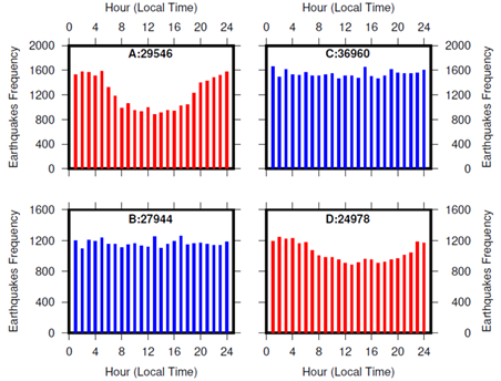
Figure 2 Hourly earthquake distribution for different small areas in the world. Red color identified earthquakes in tropical zones and blue color otherwise. Number of earthquakes in the distribution is shown in parenthesis.

Figure 3 Hourly earthquake distribution for seismic events with magnitude bigger than 4 worldwide. Red color identified earthquakes in the intertropical zone and blue color otherwise. Different period are presented for tropical earthquakes distribution. Each graph shows in parenthesis the total number of earthquakes in the distribution.
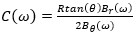
Considering the correlation that exists between the diurnal time-varying conductive response of the Earth´s interior and earthquakes (Moreno and Calais, 2021), hourly distributions of this scalar were made for different magnetic stations worldwide. In this sense, it was applied the definition for conductivity response or C-response defined by Fujii and Schultz (2002), considering a 3D electromagnetic response of the Earth. In this case, the C-response for specific location at the Earth’s surface is defined in eq. (1)
 (1)
(1)
where, B r and B Ɵ are the radial and horizontal components of the geomagnetic field, respectively, R is the Earth’s radius, Ɵ is the co-latitude of the location and ω denotes the angular frequency. Equation (1) is expressed in frequency-domain, but it was applied on time-domain because the interest is focus to time-varying C-response. The values were calculated from the hourly magnetic field average during 2020. It can be observed in Figure 5, that the diurnal variation of the conductive response at each site located in the intertropical zone (red color) has a bay-shape distribution, while the conductive responses at sites outside the tropics do not have any defined shape, sometimes approximately flat. To understand the connection between the Earth’s conductivity response and earthquakes, it is need to understand the foundation of the global atmospheric electric circuit formed between the ionosphere and the Earth’s surface (Rycroft, Israelsson and Price 2000; Williams 2009).
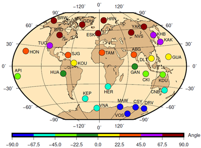
Figure 4 Angle between the magnetic flow vector and Earth’s surface for ground-based magnetic stations in the world. It was computed from horizontal and vertical components of the magnetic field during 2020.
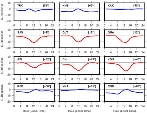
Figure 5 Diurnal variation of Earth’s conductivity response (C-response) for different locations in the world computed from magnetic field data during 2020. Angles between magnetic flow vector and Earth’s surface is shown in brackets. Curves in red color identified magnetic stations located in the intertropical zone. The scalar C is represented as the different from the maximum value.
Global atmospheric electric circuit
The atmosphere behaves like an electrical conductor because it is ionized by solar radiation. The atmospheric disturbance zones, with high activity of thunderstorms, act as a generator in the circuit, injecting electric current into the ionosphere, which then returns to the Earth's surface in fair weather zones (Figure 6). The upper atmosphere has a small electrical resistance than the lower one. In this sense, when the solar wind disturbs the geomagnetic field and injects charged particles or solar energetic particles (SEP) into the ionosphere, a variation in the electrical potential occurs within the global electric circuit, which has an electrical conductor orthogonal to the Earth's surface. Consequently, the force induced through the conductor is maximum if the angle between the magnetic flow and the electric conductor is 90 degrees, as can be seen in the definition of Laplace's force law shown in Figure 6.

RESULTS AND DISCUSSION
The diurnal variation of the electrical potential in the atmosphere is much more significant in the intertropical zone because the angle formed between the geomagnetic flow and the atmospheric electric conductor is closer to 900. On the other hand, middle latitudes and polar zones decrease significantly the angle below 450, which could explain the effect observed in the hourly earthquake distribution for each of the studied areas. It is observed from Figure 4 that tropical zones show angles between geomagnetic flow and Earth’s surface below 45 degrees, which means greater than 45 degrees for angles between the magnetic flow and the atmospheric conductor.
Furthermore, any diurnal variation in the atmospheric electrical potential will be more effective to change the electrical current flowing to the Earth’s interior when compared to middle and polar latitudes. Consequently, tectonic faults that are considered good conductors of electricity, due to increased porosity and micro-fractures in rocks, experience an electrical current greater than what they are normally exposed to. This electric current can generate a reverse piezoelectric effect, exerting an elastic deformation in rocks (Moreno and Calais 2021; Marchitelli et al. 2020).
For example, it is known that a crystal, such as quartz crystal, becomes electrically charged if it is subjected to high pressures, which is call “piezoelectric effect”, but it also oscillates or deforms when exposed to an electric current (Eccles, Sammonds and Clint 2005), which is call “reverse piezoelectric effect”. From this, it can be suggested that depending on the piezoelectric properties of minerals in rocks, these can break if they exceed the critical elastic deformation. In this sense, we are not saying that for an earthquake to occur, the existence of reverse piezoelectric effect is necessary, but rather that, these phenomena can be considered a trigger mechanism of earthquakes. The earthquakes will always occur due to the constant deformations induced by the movement of the tectonic plates, but there are trigger factors that can advance them in time. Another important aspect to take into account is the amount of samples used to make an hourly earthquake distribution. For example, taking only earthquakes greater than magnitude 5, will not appear any bay-shape hourly distribution in the intertropical zone because the samples are not statistically significant.
CONCLUSION
Diurnal earthquakes distributions are modulated by time-varying electrical potential in the global atmospheric electric circuit. The hourly earthquake frequency describes a bay-shape distribution in the intertropical zone, meanwhile earthquakes outside the tropics did not show any defined shape. The factor making the different between zones is connected with the geomagnetic flow orientation. The intertropical zone has angles between the magnetic flow vector and the atmospheric electrical conductor more close to 900 than middle latitudes and polar zones, meaning a more significant time-varying electrical potential in the global atmospheric electric circuit. Areas with angles between the geomagnetic flow vector and Earth’s surface below 450 are more susceptible to show bay-shape hourly earthquake distribution based on Laplace’s force law. Reverse piezoelectric phenomena can be considered a trigger mechanism of earthquakes.

