ORIGINAL ARTICLE

Evaluation of Methods to Calculate Dynamic Load Coefficients

MSc. Raudel Flores Moreno^{I  *} 

Dr. Gilberto de Jesús López Canteñs^I 

Dr.Cs. Arturo Martínez Rodríguez^II 

Dr. Eugenio Romantchik Kriuchkova^I 

MSc. Geisy Hernández Cuello^II 

^IUniversidad Autónoma Chapingo (UACh), Departamento de Ingeniería Mecánica Agrícola (DIMA), Texcoco, Chapingo, Estado de México, México.

^IIUniversidad Agraria de La Habana (UNAH), Centro de Mecanización Agropecuaria (CEMA), San José de las Lajas, Mayabeque, Cuba.

ABSTRACT

Dynamic forces and impact loads usually act on agricultural machines, causing breakages or failures. That is due to the nature of the impact loads, which are of short duration and decrease the capacity of the material of absorbing the deformation energy. The calculation methods that allow obtaining dynamic load coefficients require complex operations. In the present investigation, three methodologies for obtaining dynamic load coefficients were evaluated and compared: analytical method (MA), numerical simulation by the finite element method (MEF) and experimental method (Mexp). The coefficients of dynamic loads obtained from the MEF reached a relative difference that oscillated between 3.479 and 5.112%, based on the experimental results. For the analytical method, comparedto the experimental results, a relative difference between 21.820 and 27.201% was reached, which is higher than that obtained by the numerical simulation method.

Keywords: elements; dynamic efforts; Impact loads; border conditions

INTRODUCTION

Precise and scientifically justified calculations of dynamic load coefficients guarantee efficient designs and a considerable saving of materials in the manufacture of prototypes.

The determination of the stresses caused by the dynamic loads is complex depending on factors such as contact area in the impact and the variation process of the contact forcesas a function of time. In this sense, most dynamic cases are quantify experimentally and for simple calculations, equivalent static charges are used. The determination of the coefficients of dynamic loads in structures subjected to impact actions, using analytical methods, represents a challenge due to their high complexity.

The method of finite elements, as a numerical method of computer-assisted discretization, is an alternative way to the analytical method of continuous medium analysis, which facilitates the solution of complex engineering problems, being considered a tool of undoubted practical value and great application worldwide. There are important results derived from the use of this method, among them the ones reported by ^{Martínez et al. (2007)}; ^{Liu et al. (2013)} and ^{Untaroiu et al.(2013)}. Also, those referred by ^{Vavalle et al. (2013)}; ^{Feng & Aymerich (2014)}; ^{Nadal et al. (2014)}; ^{Zhanbiao et al. (2014)}; ^{Singh & Singh (2015)}; ^{Zhao et al. (2015)}; ^{Kong et al. (2016)}; ^{Xiaofei et al.(2016)} and ^{Castro & Güiza (2017)}.

The objective of this work was to evaluate and compare three methodologies for determining dynamic load coefficients: the traditional analytical method (MA), the numerical simulation based on the finite element analysis (MEF) and the experimental method (Mexp), taking this last as a comparison and validation pattern of the theoretical methods.

METHODS

A multifactorial type design was used, using two factors as independent variables that correspond to the height and the impact load, with ten and three levels, respectively. The impact height levels were from 0 to 1 m with intervals of 0.1 m and the load levels were 25; 400 and 800 N.

For the three methods analyzed, the coefficient of dynamic loads was determined starting from the determination of the static deflection produced on a mechanical system taken as an object of study under the action of static charges with a magnitude equal to the weight of a body that impactsince a certain height. Once the maximum static deflections of the system under study were determined, the coefficient of dynamic loads was determined using the expression according to ^{Pisarenko and Yakovlev (1979)}:

$kd=1+\sqrt{1+\frac{2H}{{\delta }_{est}}}$ (1)

where:

kd	- Coefficient of dynamic loads;
δ est	- Deflection or maximum static arrow, which also depends on the solicitation scheme and the support conditions;
H	- Height of fall of the body that impacts on the system under study.

In this work, the static deflection of the system under study was determined by the three mentioned methods: the traditional analytical method of the mechanics of materials; the method of finite elements and the experimental method.

Description of the Mechanical System under Study

As a study object, a beam of square cross section (Table 1) was used in horizontal position and supported at its ends with a joint and a simple support, as shown in Figure 1. In the center of the beam, three levels of load Q (25, 400 and 800 N) were applied to provoke different levels of static deflections (δ). In Table 2, the mechanical properties of the material are shown.

TABLE 1 Description of the system under study 

Cross section	Side, mm	Mass, kg	Moment of inertia, m^4	Length, mm	Acting load, N
Square	39.09	12	1.95*10^-7	1000	From 25 to 800 at the interval of 25

FIGURE 1 Descriptive scheme of the system under study. 

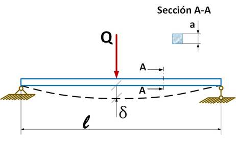
TABLE 2 Physical mechanical properties of the beam material 

Description	Value
Modulus of elasticity	200 000 MPa
Poissoncoefficient	0.29
Density of mass	7900 kgm^-3
Limittotraction	420.507 MPa
ElasticLimit	351.561 MPa

Source: ^{Warrendale (2001)}

Determination of Static Deflections by the Traditional Analytical Method

For the case under study, consisting of a horizontal beam simply supported when the application of the load is made in the center of the beam and the maximum static arrow is given by the expression:

${\delta }_{est}=\frac{Q{l}^3}{48EJ}$ , [m] (2)

where:

Q	- mg: weight of the impacting element, kg ms^-2
l	- length of the beam, m
E	- modulus of elasticity of the beam material
J	- moment of inertia of the section of the beam

FIGURE 2 Convergence analysis to determine the characteristics of the mesh. 

From the element size, the rest of the properties of the mesh are established (Table 3). In Figure 3, a 3D view of the model of the beam with the resulting meshing and boundary conditions is shown, where the restrictions (green arrows) and the statically applied load (red arrows) are represented.

TABLE 3 Characteristics of the mesh used in the analysis 

Parameters	Mesh	Quality	Tolerance	Number of nodes	Number of elements	Size of elements
Description	Solid, Standard	High	0.05 mm	4,340	2,342	20 mm

FIGURE 3 3D model of the beam with the representation of the boundary conditions. 

Description of the Experimental Method Used

The experimental determination of the static deformations that allowed determining the coefficients of dynamic loads of the system studied, under different dynamic loads, was carried out by means of electrical extensometry techniques.

On the underside of the center of the beam studied,strain gauges were placed (Figure 4) configured in a quarter of Wheatstone bridge, with the aim of obtaining voltage signals proportional to the unitary deformation (considering the deformations within the elastic limit of the material), produced by static charges of different magnitude. The static charges were obtained by placing weights of 25 N; 400 N and 800 N in the center of the beam and recording the output voltage (eest) of the measurement system. In a similar way, the output voltage (edin) produced by the same applied loads was recorded, dropping the same weights from different heights between 0.1 and 1 m to the center of the beam. For each treatment, three repetitions were made. The quotient of the voltages obtained, for each of the loads and heights applied, allowed obtaining the coefficient of dynamic loads in each case, applying the expression:

$k_d=\frac{e_{din}}{e_{est}}=\frac{{\epsilon }_{din}}{{\epsilon }_{est}}=\frac{{\sigma }_{din}}{{\sigma }_{est}}$ (3)

where

eest	- is the voltage registered under the action of the loads applied in static form;
e din	- is the maximum voltage under the action of the loads applied dynamically (when dropping the weights from different heights);
ε est and ε din	- are the unit deformations corresponding to the static and dynamic loads, respectively;
σ est and σ din	- are normal stresses corresponding to static and dynamic loads, respectively.

FIGURE 4 Strain gages stuck on the underside of the beam. 

The signals coming from the strain gauges (of the order of the mV), were processed in a dynamic amplifier, model KYOWA-YA-520 with amplification modules of type DPM-602B, being amplified up to voltage levels between ± 5V.

The analog signal coming from the amplifier (Figure 5) was digitalized in an analog-digital converter model NATIONAL INSTRUMENTS - NI USB-4431 and introduced at a rate of 100 samples per second in a laptop computer for further statistical processing.

FIGURE 5 Diagram of the instrumentation used during the registration of the signals proportional to the deformation of the beam. 

RESULTS AND DISCUSSION

Figure 6 shows one of the outputs of the static analysis by the MEF to determine the unit deformation of the beam under study. When the beam is subjected to 800 N static load, it is observed that the value of the unit strain is 86.976 μstrain, while the result of the stress for that same load value is shown in Figure 7, where it reached a value of 17.3952 MPa.

FIGURE 6 Deformations in the center of the beam under the action of a static load of 800 N. 

FIGURE 7 Stress in the center of the beam under the action of a static load of 800 N. 

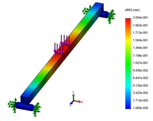
FIGURE 8 Deflection of the beam in the vertical direction for a static load of 800 N by analysis with the finite element method. 

Experimental Evaluation of the Numerical Simulation

Figure 9 shows two graphs with the cumulative distribution of the deformations predicted with the model analyzed by the MEF and the experimental results. The data obtained showed that the maximum distance between the accumulated distributions of the two samples is 0.03125 μstrain, where the approximate p-value obtained is greater than 0.05, so there is no statistically significant difference between the two distributions for a confidence level of 95%. It was observed that the data obtained for the stresses predicted with the model analyzed by MEF and those calculated from experimental tests coincide with the results obtained for the deformation, this is because the stresses are calculated from the deformations using the law of Hooke.

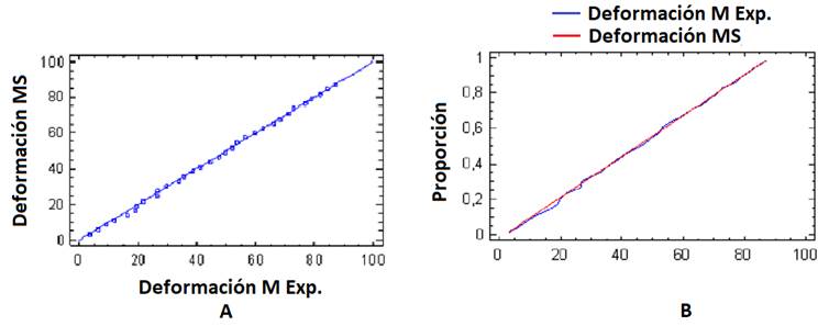
FIGURE 9 Accumulated distribution (A) and distribution function (B) between the deformations predicted by the simulation and those obtained experimentally. 

Figure 10 shows the cumulative distribution graph to compare the deflections predicted with the model analyzed by MEF and the experimental results, which shows that the maximum distances between the accumulated distributions of the two samples are of 0.09375 mm. For the behavior of the predicted and experimental deflection values, an approximate p-value of 0.998965 was obtained. Since it is greater than 0.05, there is no statistically significant difference between the two distributions for a 95% confidence level.

FIGURE 10 Accumulated distribution (A) and distribution function (B) between deflections predicted by the simulation and those obtained experimentally. 

Result of the Coefficients of Dynamic Loads by the Three Methods Studied

Table 4 shows the results of the determination of the dynamic load coefficients by the different methods studied and the relative difference between the methods and the experimental results. It can be seen that the relative difference of the MEF ranged between 3.479 and 5.112%, being substantially lower than the values ​​obtained by the analytical method (MA), which ranged from 21.820 to 27.201%.

The dynamic load coefficients reached values ​​of 391.203 for the analytical case (MA), of 501.001 for the experimental case and a value of 528.047 for when the dynamic load coefficients were calculated from the data obtained via numerical simulation by the method of the finite elements (MEF), with a load of 25 N. The highest values ​​of the coefficients of dynamic loads in the three calculation methods were recorded for the highest height studied (1 m) and with the lowest of the loads applied (25 N). For the same impact height it was determined that the highest values ​​of dynamic load coefficients were recorded for the lower mass impact loads (25 N). At the same impact height, the lowest dynamic load coefficients were obtained while the impact load was greater. The case that the highest coefficient values ​​of dynamic loads were recorded for the lower load is because the increase in the mass of the hitting element causes greater deflections, therefore, the coefficient of dynamic loads decreases, due to its inversely proportional relationship.

TABLE 4 Relative differences of the dynamic load coefficients by both methods métodos 

Impactheight; m	Impact load; N	Coefficients of dynamicloads			Relativedifference
		(MA)	(M Exp.)	(MEF)	MA-MExp; %	MEF- MExp; %
0.1	25	124.397	159.117	167.62	21.820	5.344
	400	31.864	42.897	45.141	25.720	5.231
	800	23	31.099	32.22	26.043	3.605
0.2	25	175.51	224.61	236.704	21.860	5.384
	400	44.637	60.243	63.417	25.905	5.269
	800	32	43.555	45.141	26.530	3.641
0.3	25	214.725	274.863	289.677	21.879	5.390
	400	54.44	73.555	77.441	25.987	5.283
	800	38.794	53.115	55.057	26.962	3.656
0.4	25	247.787	317.229	334.335	21.890	5.392
	400	62.704	84.777	89.265	26.037	5.294
	800	44.637	61.174	63.417	27.033	3.667
0.5	25	276.916	354.555	373.679	21.898	5.394
	400	69.986	94.664	99.682	26.069	5.301
	800	49.785	68.275	70.782	27.082	3.672
0.6	25	303.251	388.3	409.25	21.903	5.395
	400	76.569	103.603	109.1	26.094	5.306
	800	54.44	74.694	77.441	27.116	3.678
0.7	25	327.468	419.331	441.96	21.907	5.396
	400	82.623	111.823	117.76	26.113	5.309
	800	58.72	80.598	83.565	27.145	3.681
0.8	25	350.009	448.215	472.406	21.910	5.397
	400	88.258	119.474	125.821	26.128	5.312
	800	62.704	86.093	89.265	27.167	3.684
0.9	25	371.468	475.343	501.001	21.853	5.398
	400	93.55	126.66	133.393	26.141	5.316
	800	66.446	91.254	94.618	27.186	3.686
1	25	391.203	501.001	528.047	21.916	5.398
	400	98.556	133.457	140.554	26.151	5.318
	800	69.986	96.136	99.682	27.201	3.689

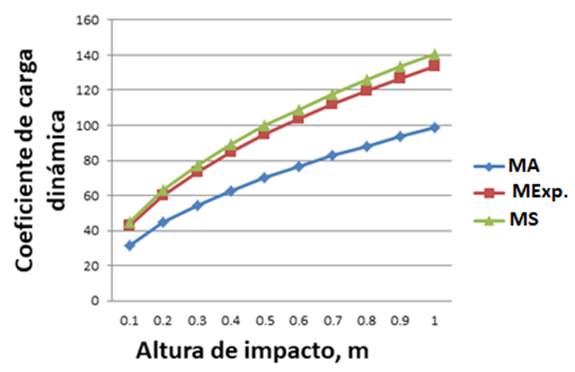
Figure 11 shows the behavior of the dynamic load coefficients by the three methods studied for an impact load of 400 N. The range of impact heights was from 0.2 to 1 m. It is observed that the behavior curve obtained by the MEF was the closest to that obtained by MExp. The results obtained by numerical simulation (MEF), gave better results and this is due to the advantage that the finite elements method offers before the analytical methods, which allows simulating the system more realistically, taking into account a greater number of factors during the simulation. The analytical processes are simplified and they are of great practical value to design innumerable systems, but theydo not allow knowing the detailsof the structural behavior under real actions.

Coinciding with the results obtained, ^{Aparicio & Casas (1987)}point out that in the interpretation of the results of tests of impact loads, it is important to know aspects that are not considered in the analytical studies. It is also vital to know the details of the phenomenon when they take into account the deflection of automobile structures to see their impact on the comfort and safety of passengers (^{Álvarez et al., 1983}). On the other hand, ^{Beltrán and Cerrolaza (1989)}, state that it is necessary to resort to more sophisticated calculation models that allow reproducing more accurately the real behavior of different systems.

FIGURE 11 Behavior of dynamic load coefficients for a load of 400 N. 

CONCLUSIONS

• The numerical simulation compared with experimental data for deformations and stresses reached a p-value greater than 0.05, so there was no statistically significant difference between the two distributions for a confidence level of 95%.

• For the deflections predicted through the model analyzed by MEF and the experimental results, an approximate p-value of 0.99 was reached, so there was no statistically significant difference between the two distributions.

• The relative difference between the coefficients of dynamic loads by experimental method (MExp.) and by numerical simulation (MEF) ranged between 3.479 and 5.122%, being substantially lower than the values obtained by the analytical method (MA), which reached values from 21.820 to 27.201%.

REFERENCES

ÁLVAREZ, R.; MOLINA, R.F.J.; DOBLARÉ, C.M.; ALARCÓN, E.: “Interacción dinámica vehículo-vía-estructura-cimiento en puentes de ferrocarril”, En: Anales de Ingeniería Mecánica, Ed. Asociación Española de Ingeniería Mecánica; Universidad de Cantabria (Dpto, vol. 1, pp. 451-460, 1983, ISBN: 0212-5072.

APARICIO, A.; CASAS, J.R.: “Resultados y conclusiones de las pruebas efectuadas en el paso superior de Alfonso X, en el Cinturón de Ronda de Barcelona: Una fuente de enseñanza”, Hormigón y acero, 162: 33-141, 1987.

BELTRÁN, F.; CERROLAZA, M.: “Análisis dinámico de estructuras sometidas a cargas no lineales”, Revista internacional de métodos numéricos para cálculo y diseño en ingeniería, 5(4): 473-502, 1989, ISSN: 1886-158X.

CASTRO, D.; GÜIZA, R.: Análisis del efecto de una grieta en el comportamiento estructural de una biela usando FEA, ser. Engineering Sciences [physics]/ Mechanics [physics.med-ph]/ Mechanics of the structures [physics.class-ph], Inst. Grupo de Investigación en Energía y Medioambiente (GIEMA). Universidad Industrial de Santander, Colombia, Colombia, 2017.

FENG, D.; AYMERICH, F.: “Finite element modelling of damage induced by low-velocity impact on composite laminates”, Composite Structures, 108: 161-171, 2014, ISSN: 0263-8223, DOI: https://doi.org/10.1016/j.compstruct.2013.09.004.

KONG, Y.S.; ABDULLAH, S.; OMAR, M.Z.; HARIS, S.M.: “Failure assessment of a leaf spring eye design under various load cases”, Engineering Failure Analysis, 63: 146-159, 2016, ISSN: 1350-6307, DOI: https://doi.org/10.1016/j.engfailanal.2016.02.017.

LIU, T.; FLECK, N.A.; WADLEY, H.N.G.; DESHPANDE, V.S.: “The impact of sand slugs against beams and plates: Coupled discrete particle/finite element simulations”, Journal of the Mechanics and Physics of Solids, 61(8): 1798-1821, 2013, ISSN: 0022-5096, DOI: https://doi.org/10.1016/j.jmps.2013.03.008.

MARTÍNEZ, R.A.; BOZA, M.Y.; LASTRA, M.D.; BARROSO, P.P.: “Análisis modal del sistema fruto-pedúnculo del Nim”, Revista Ciencias Técnicas Agropecuarias, 16(3): 43-46, 2007, ISSN: 1010-2760, e-ISSN: 2071-0054.

NADAL, E.; RÓDENAS, J.J.; SÁNCHEZ, O.E.M.; LÓPEZ, R.S.; MARTÍ, P.J.: “Sobre la utilización de códigos de elementos finitos basados en mallados cartesianos en optimización estructural”, Revista internacional de métodos numéricos para cálculo y diseño en ingeniería , 30(3): 155-165, 2014, ISSN: 0213-1315, DOI: https: //doi.org/10.1016/j.rimni.2013.04.009.

PISARENKO, G.S.; YAKOVLEV, A.P.: Manual de resistencia de materiales, Ed. Mir Publishers, Primera ed., Moscú, Rusia. URSS, 1979.

SINGH, N.K.; SINGH, K.K.: “Review on impact analysis of FRP composites validated by LS‐DYNA”, Polymer Composites, 36(10): 1786-1798, 2015, ISSN: 0272-8397, DOI: 10.1002/pc.23064.

UNTAROIU, C.D.; YUE, N.; SHIN, J.: “A finite element model of the lower limb for simulating automotive impacts”, Annals of biomedical engineering, 41(3): 513-526, 2013, ISSN: 0090-6964, DOI: 10.1007/s10439-012-0687-0.

VAVALLE, N.A.; MORENO, D.P.; RHYNE, A.C.; STITZEL, J.D.; SCOTT, G.F.: “Lateral impact validation of a geometrically accurate full body finite element model for blunt injury prediction”, Annals of biomedical engineering , 41(3): 497-512, 2013, ISSN: 0090-6964, DOI: https://doi.org/10.1007/s10439-012-0684-3.

WARRENDALE, P.A.: SAE Handbook. Society of Automotive Engineers, Warrendale P.A.: Metals Handbook. American Society for Metals. Materials Park. Ohio, USA., 2001.

XIAOFEI, W.; YINGCHUN, S.H.; XIANDONG, L.; WANG, H.; JIEGONG, W.: “Simulation of biaxial wheel test and fatigue life estimation considering the influence of tire and wheel camber”, Advances in Engineering Software, 92: 57-64, 2016, ISSN: 0965-9978, DOI: https://doi.org/10.1016/j.advengsoft.2015.11.005.

ZHANBIAO, L.; DI CECCO, S.; ALTENHOF, W.; THOMAS, M.; BANTING, R.; HU, H.: “Stress and fatigue life analyses of a five-piece rim and the proposed optimization with a two-piece rim”, Journal of Terramechanics, 52: 31-45, 2014, ISSN: 0022-4898, DOI: https://doi.org/10.1016/j.jterra.2014.02.002.

ZHAO, Y.Q.; ZANG, L.G..; CHEN, Y.Q.; LI, B.; WANG, J.: “Non-pneumatic mechanical elastic wheel natural dynamic characteristics and influencing factors”, Journal of Central South University, 22(5): 1707-1715, 2015, ISSN: 1005-9784, DOI: https://doi.org/10.1007/s11771-015-2689-1.

Received: December 12, 2018; Accepted: September 02, 2019

^*Author for correspondence: Raudel Flores Moreno: e-mail: [e-mail]

Raudel Flores Moreno, Applicanttodoctorate, Universidad Autónoma Chapingo (UACH), Programa de Ingeniería Agrícola y Uso Integral del Agua, Departamento de Ingeniería Mecánica Agrícola (DIMA, km 38.5 carr. México - Texcoco. CP 56230, Chapingo, Estado de México, México, e-mail: [e-mail]

Gilberto de Jesús López Canteñs, Docente, Universidad Autónoma Chapingo (UACH), Programa de Ingeniería Agrícola y Uso Integral del Agua, Departamento de Ingeniería Mecánica Agrícola (DIMA, km 38.5 carr. México - Texcoco. CP 56230, Chapingo, Estado de México, México, e-mail: [e-mail]

Arturo Martínez Rodríguez, Profesor e Investigador Titular, Universidad Agraria de La Habana (UNAH), Centro de Mecanización Agropecuaria (CEMA), San José de las Lajas, Mayabeque, Cuba, C.P: 32700, e-mail: [e-mail]

Eugenio RomantchikKriuchkova, Docente, Universidad Autónoma Chapingo (UACH), Programa de Ingeniería Agrícola y Uso Integral del Agua, Departamento de Ingeniería Mecánica Agrícola (DIMA, km 38.5 carr. México - Texcoco. CP 56230, Chapingo, Estado de México, México, e-mail: [e-mail]

Geisy Hernández Cuello, Investigadora Auxiliar, Universidad Agraria de La Habana (UNAH), Centro de Mecanización Agropecuaria (CEMA), San José de las Lajas, Mayabeque, Cuba, C.P: 32700, e-mail: [e-mail]