


 Servicios personalizados
 Inglés (pdf)
 Articulo en XML
 Referencias del artículo
 Enviar articulo por email
 Citado por SciELO
  Similares en
SciELO
Similares en
SciELO 
 Permalink
Introduction
The pharmaceutical industry is one of the economic and health strategic sectors of the world nowadays. This industry has the mission of ensuring better living standards and contribute to increase the life expectancy of those who suffer illnesses and of the population in general. It is a stepping stone for those who fight for preventing, diagnosing and treating diseases every day. The decisive role of this sector has been reinforced with the appearance, transmission or infection of the new SARS-CoV-2 in human beings, which causes the COVID-19. Due to that, this sector, as well as the biotechnological one, is in charge of the development of a vaccine to control the infection; it plays a key role in reducing the number deaths and producing diverse medications which are necessary to attack the symptoms of the pandemic, thus avoiding deterioration of the patients’ health and the complications that appear in patients who suffer from other pathologies.
One of the methods that shed light on the implementation of the medications inventory planning process is demand forecasting, which is an integral part of business process management. Despite the complexity and execution of forecasting processes across different businesses, the intended purpose stays the same: obtaining a fairly accurate estimation of future demand for a product or service given historical data and the current state of the environment (e.g., political, social, economic) to plan and organize businesses accordingly. Forecasting accuracy is still a big challenge in the pharmaceutical industry (Merkuryeva, et al., 2019).
Accordingly, Access to medications is essential for materializing access to health as a fundamental human right. As such, it is included in the United Nations Sustainable Development Goals, and is recognized as key-element for scaling-up access to health services towards universal health coverage. Pharmaceutical services are not restricted to the logistical component of medications availability. They also include management and quality of services, and promotion of adequate use of medications. Even though, the availability of medications is an extremely important dimension for the assurance of access to these products (Mota Soares, et al., 2019).
In today’s organizations, which are subject to abrupt and enormous changes that affect even the most established of structures and where all requirements of business sector need accurate and practical reading into future, the forecasts are becoming very crucial since they are the sign of survival and the language of business in the world. A forecast is a science of estimating the future level of some variables. The variable is most often demand, but it can also be something else, such as supply or price. Forecasting is the operation of making assumption about the future values of studied variables (Fattah, et al., 2018).
A variety of forecasting methods have been developed based on two well-known approaches to forecasting: qualitative and quantitative. Correspondingly, qualitative methods such as executive opinions, Delphi technique, sales force polling and customer services generate forecasts based on judgements or opinions, while quantitative techniques may be grouped under historical data forecasts, e.g., naive method, trend analysis, time series analysis, Holt’s and Winter’s models, or under the so called associative forecasts which identify causal relationships between variables using simple, multiple or symbolic regression. In addition, mixed or combined models enable integration of both approaches. In the pharmaceutical industry, time-series models are used most often (52%) and causal models account for 24%, while judgmental - for 19% and remaining 5% represent mixed or combined models (Merkuryeva, et al., 2019).
During the last decade, few mathematical methods have been presented to forecast the medications demand or the morbidity of a specific illness, which could also be useful in such task. In this paper, the search of bibliographic sources was done in databases such as: Scopus, Scielo, PubMed, Inbiomed and Virtual Health Library and Web of science. Some of the articles consulted are those of Ren, et al. (2013), who presented a combined model, ARIMA-BPNN (back propagation neural network) to forecast the incidence of hepatitis E in Shanghai. This combination of both models was introduced in order to overcome the main limitation of the ARIMA, that is to say its pre-assumed linearity. The goodness-of-fit of the ARIMA model proposed by the authors were: the stationary R 2 , the root mean square error (RMSE), the Bayesian information criterion (BIC), the Ljung-Box Q statistics. It was also used the mean error rate (MER) to explain the comparison of predicted and actual values between single ARIMA and ARIMA-BPNN. Merkuryeva, et al., (2019), who have proposed an experimental analysis of three forecasting scenarios, concluding that the symbolic regression-based forecasting model provides the best fitting curve to history demand data and the lower error estimates across all scenarios, as well as the ability to more accurately predict demand peak sales in their study. In this case, the Pearson 𝑅 2 coefficient is used to measure fitness. Roosa, et al. (2020), who have developed three phenomenological models used previously to derive short-term forecasts in other epidemics. These are: The generalized logistic growth model (GLM), the Richard’s model and a sub-epidemic wave model. The criteria used by these authors to assess the visual fit of the models were the residuals and the mean squared error (MSE). Linnér, et al. (2020), compared the predicted pharmaceutical expenditure with actual expenditure, including medications used in hospitals and dispensed prescription medications. A linear regression model was used and fitted to a time series of drug utilization data. Yonar, et al., (2020), presented the forecasting models used by Germany, United Kingdom, France, Italy, Russian, Canada, Japan, and Turkey to estimate the number of COVID 19 epidemic cases between 1/22/2020 and 3/22/2020. The models approached by these authors are: regression models (cubic models), which resulted to be the best for all countries and the Box-Jenkins and exponential smoothing models, concluding that could be used because of having a Mean Absolute Percentage Error (MAPE) less than 10%.
This paper presents a procedure to forecast the demand of one of the 487 medications studied in a pharmaceutical organization, as well as evaluating the results and the goodness-of-fit of the model selected, presenting the forecast done for the period of time of 144 months, from January 1st, 2009 to December 31st, 2020. The rest of this paper is organized as follows. In section 2, the materials and methods are presented. In section 3, the results and discussion are shown. The conclusions are also presented after section 2.
Materials and methods
The data used in this paper contain the number of blisters sold of the item selected during 144 months, from January 1st, 2009 to December 31st, 2020. The item is labeled as AZ123. Data is modeled to forecast its needs for each of the months of 2021. The forecasting is compared with the morbidity data obtained from pharmaceutical authorities and then adjusted if necessary. Different forecasting models were tentatively tested, then the best goodness-of-fit model, ARIMA (0,1,1)x(0,1,1)12, is selected. Historical data is processed by the IBM SPSS Statistics for Windows, Version 23.0. The series was divided in two parts, data from January 1st, 2009 to data from December 31st, 2019 were used to perform the time series model and data from January 1st, 2020 to data from December 31st, 2020 were used to check the adequacy of the model. The quantitative approach was used, as well as the problem-solving scientific method.
The inventory selected is a drug stock, mainly because these articles have a direct impact on the living standards of society, and due to the fact that its significance has been more tangible these days, in which the occurrence of the COVID-19 pandemic, caused by the SARS-CoV-2, has reinforced the need of the development of a strong planning system for this kind of inventory. These facts have been exposed by Bond & Newton (2020), who have mentioned that the ocurrence of drug shortages for the treatement, diagnosis and prevention of COVID-19 and of other diseases have been evident, in some cases because the pharmaceuticals applied for the treatment of those other illnesses and their symptoms have been used for the treatment of the symptoms and complications which the patients suffering from COVID-19 have needed. Otherwise, the forecasting models which are theoretically explained can be applied in other kinds of inventory too, by taking notice of their historical behaviour, trends, seasonality and other aspects which be taken account of in this type of study.
Among the models which are mostly used to forecast a demand meet the exponential smoothing models: simple smoothing, Brown/Holt linear exponential smoothing, weighted moving averages, Winters´ additive, Winters´ multiplicative and simple seasonal. Some other models and methods have also added to this task, such as the neuronal networks and the autoregressive integrated moving average (ARIMA) models, which have been also used to forecast the number of COVID 19 epidemic cases in many countries. This fact is evidenced by Yonar, et al., (2020).
The procedure designed consists of three main stages: the first one is the collection and organizing of data; the second one, the selection of the model, the third one is related to the adjusting of the forecasting and the fourth one is the forecasting accuracy.
First stage: data collection and organization
Data are collected from the historical records of the pharmaceutical organization where the study took place. Data collected are adjusted from considering the shortages occurred during the period selected and they are obtained from the records enable for this purpose. Data are entered in an Excel spreadsheet and organized according to the demand occurred in each of the 144 months.
Second stage: selection of the forecasting model
The first step in analyzing a time series is the graphical representation, through the sequence plot and the simple and partial autocorrelation functions, of the variable over time. This representation shows the possible trend of the series, as well as the existence or not of seasonal and stationary components. In the same way, outliers are detected, which should be adjusted to improve the series and thus obtain a more reliable model.
The selection of an ARIMA forecasting implies the development of four phases or steps, according to the Box-Jenkins methodology, as shown in figure 1
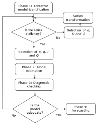
Phase 1: Tentative model identification
The first phase is addressed to tentatively identify the model by running a plot of data, determining the stationarity condition of the original series 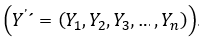 .
.
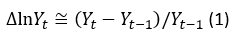
In this phase, it is determined if the data of the series are stationary, since the ARIMA models are designed for this type of data. The stationarity is determined by analyzing the sequence plot, the mean-standard deviation plot and the autocorrelation function (ACF) and the partial autocorrelation (PACF) are also built and analyzed. If differencing is necessary, the series is transformed by applying logarithms, in the way expressed in equation 1.
The Box-Jenkins methodology is widely used for time series analysis and includes ARIMA models applied to the series that are non-stationary but are made stationary with the operation of differencing the series. The base of Box-Jenkins methodology is to choose an ARIMA model that includes the most suitable but limited parameter among the various model options, depending on the nature of the considering data (Yonar, et al., 2020).
ARIMA (p, d, q) models are obtained by taking the difference of the series from d degree and adding it to an ARMA (p, q) model for the stabilizing the process. In the ARIMA (p, d, q) models, p is the degree of the autoregressive (AR) model, q is the degree of the moving average (MA) model and d stands how many differences are required to make the series stationary. ARIMA model becomes AR (p), MA(q) or ARMA (p, q) if the time series is stationary (Yonar, et al., 2020).
The mathematical expression on an ARMA (p, q) model is as shown in equation 2:

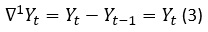
The first difference of the non-stationary Yt is calculated by using the mathematical expression 3:
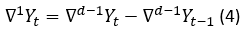
If the  is not still stationary, the difference taking process is repeated for the d times until being stationary (Yonar, et al., 2020). The expression which represents this process is shown in the equation 4.
The expression of ARIMA (p, d, q) is as shown in equation 5.

Where,
|
the parameter values for autoregressive operator, |
|
the error term coefficient, |
|
the parameter values for moving average operator, |
|
the time series of the original series differenced at the degree d. |
The Seasonal Auto-Regressive Integrated Moving Average (SARIMA) models are more adequate for long-term than for short-term predictions with seasonal patterns. However, these latter are analyzed on a seasonal series, and require at least 50 data. The SARIMA model is useful in situations in which the data of seasonal series show periodic seasonality fluctuations that repeat themselves with almost the same intensity every year (Rojas, et al., 2019).
A SARIMA seasonal model with s observations per period, denoted by (p, d, q) X (P, D, Q)s is given by the expression 6.
 (Rojas, et al., 2019) (6)
Where,
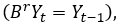
B: |
is the delay operator |
Yt: |
is the time series of variable Y in time t, |
t,: |

|
And the autoregressive polynomial (AR) of the non-seasonal part, of the order p, is symbolized with and  is developed as follows, in equation 8.

Whereas is the polynomial of moving averages (MA) of the seasonal part Q order, where:

And 𝜃 𝐵 is the polynomial of moving averages (MA) of the non-seasonal part of the q order,
where:

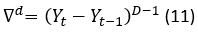
The number of differences needed to make stationary the series in the non-seasonal part, is symbolized as d and calculated as shown in the expression 11.
whereas D is the number of seasonal differences and it is represented as shown in expression 12.

 refers to the terms of random error, also called white noise, which are assumed to be random variables, independently distributed in identical manner, sampled from a distribution with a mean of zero and a variance expressed as:
  .
.
Besides looking at the graphical presentation of the time series values over time to determine its stationary or non-stationary condition, the sample ACF also gives visibility to the data. Non-stationary data displaying trend behavior can be transformed through regular differencing (Tshepiso Tsoku, et al., 2017).
Phase 2: Model estimation
The model estimation phase involves estimation of the parameters of the models identified in the first phase. The least squares approach is employed in model estimation (Tshepiso Tsoku, et al., 2017).
Once the model has been tentatively identified, its parameters are estimated. If d differences have been taken in the series, d observations will be lost, leaving T-d data available for estimation. In this process the following hypotheses must be verified:
Hypothesis 1:
 has a white noise structure and follows a Normal distribution of mean 0 and variance σ^2
Hypothesis 2:
H 0 : the autoregressive part (AR) is stationary.
Hypothesis 3:
H 0 : the seasonal part (MA) IS invertible.
Phase 3: Diagnostic checking
Diagnostic checking is the third phase, and in the Box-Jenkins methodology, essentially involves the statistical properties of the error terms (normality assumption, weak white noise assumption) as well as common testing procedures on the estimates. 𝜀 𝑡 is expected to follow a white noise process. Graphical procedure and formal testing procedure can be used to test adequacy of the model. In the graphical procedure, a plot of the residuals is examined to check for outliers (Tshepiso Tsoku, et al., 2017). To check the overall acceptability of the overall model, the Ljung-Box test can be used as follows:
H 0 : the model is adequate versus H 1 : the model is inadequate.
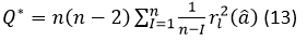
The test statistics Q* is calculated by using the expression 13.
Where,

is the number of observations,
 is the degree of non-seasonal differencing used to transform the original time series values into stationary,
 is the square of the autocorrelation of the residuals at lag l.
If the p-value is greater than significant level 𝛼 or equivalently Q* is less than chi-square distribution, the null hypothesis cannot be rejected, concluding that the model is adequate. If a model is rejected at this stage; the model-building cycle has to be repeated (Tshepiso Tsoku, et al., 2017).
Phase 4: forecasting
Forecasting is the final and most important stage of the Box-Jenkins process. There are two broad
types of forecasts: one step ahead forecasts are generated for the next observation only when multi-step ahead forecasts are generated for 1,2, 3...,s steps ahead. Many researchers suggest that Box-Jenkins’ ARIMA is the most accurate forecasting model. ARIMA wins over other models, Holt’s forecast model and a combination of Box-Jenkins and Holt’s in regression, by providing lowest mean MAPE. There are many simple measures of prediction accuracy, for instance the mean squared error (MSE), mean absolute error (MAE) and mean squared deviation (MSD) (Tshepiso Tsoku, et al., 2017).
The MAPE is calculated by using the expression 14.
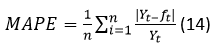
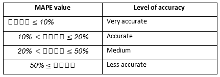
This test statistic can be used to compare the accuracy of forecasts based on two entirely different series. The level of accuracy for the MAPE test is divided into four stages. Each level of accuracy gives the percentage of the accuracy of a predicted value compared to the original time series value (Tshepiso Tsoku, et al., 2017).
The table 1 shows the level of accuracy for MAPE test.
3- Third stage: adjusting of the forecasting
In this stage the forecasting obtained is adjusted to the morbidity changes that could be recorded by the pharmaceutical authorities during the planning process. So that, the final forecasting reflects the most accurate behaviour of the variable studied for the next period.
4- Fourth stage: forecasting accuracy
The forecasting accuracy refers to the further actions which should be carried out in the future to check up on the real behavior of the demand in the next period for which the forecasting was performed. The accuracy of the model is measured as shown in equation 15.
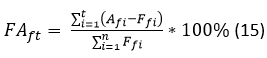
Here,
FA ft : |
denotes the forecasting accuracy of the model for the item (f) in a period (t). |
i: |
represents a single period, e.g. a week, a month and a year. |
A fi : |
denotes de actual demand behaviour for the item (f) in the period (i). |
F fi : |
stands for the demand forecasting of the item (f) in the period (i). |
Results and discussion
This section expounds the results obtained in every stage of the research process.
First stage: data collection and organization
Historical data of demand of the item labeled as AZ123 is collected from the commercial records of the pharmaceutical organization. Then, they are entered in an Excel spreadsheet. The quantities of blisters sold are organized by months, according to the moment in which the sale occurred. Once ordered, historical data are adjusted, for the first time, by considering the unrecorded demand, due to shortages in the supply chain. This information is obtained from the technical department of the pharmaceutical organization. Once the adjustments have been made, the data is exported to the statistical software SPSS, version 23.0.
Second stage: selection of the forecasting model
The selection of the forecasting model is carried out through the phases of the Box-Jenkins methodology, which are developed below.
Phase 1 and 2: Tentative model identification and model estimation
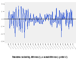
First, it is checked whether the series is stationary or not. So the sequence plot is built as shown in figure 2.
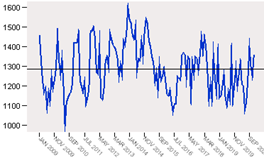
As it can be observed, the series shows various peaks, some of which appear to be equally spaced and some others do not. The peaks equally spaced suggest the presence of a periodic component to the time series. This seasonal pattern should be associated to the periods of time in which the presence of some diseases and their symptoms are treated with the pharmaceutical studied. It can also be noticed that there are some points between June, 2014 and December, 2014 which indicates that some data have significant deviations from the neighboring data points. It is also evident that the distance between peaks, in some cases, is not regular, which is indicative of an unsteady variance and an inconstant mean.
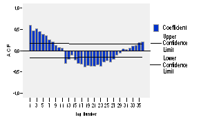
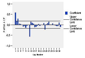
The correlograms of the original series are also built (see figures 3 and 4), which allows to know about whether the series is stationary and tentatively determine the possible model to be applied.
When observing the figure 3, it could be presumably assumed that the series follows an annual seasonality, due to significant peaks at the lags of 12, 24 and 36, and it is also noticeable that this function does not dwindles, so it could be assumed that it is not stationary.
When analyzing the partial autocorrelations in figure 4, it is evident that such significance only appears at the lag of 24, which makes unsure the possibility of the abovementioned seasonality.
Taking into account the no equally spaced peaks, the distance differences between some of these spikes and the doubt about seasonality; firstly, a mean and a variance analysis is carried out by applying a report in columns, in order to verify the possible unsteady behaviour of the series variance and the inconstant mean; whose results, shown in the table 2, confirm that data have different means and variances for each of the 12 years taken into account. Due to this fact, a natural logarithmic transformation is applied to the series, as well as one difference in order to make the series steady in variance and constant in mean, that is to say to make the series stationary in both parameters.
Table 2 - Report in columns.
| Year | Mean | Variance |
|---|---|---|
| 2009 | 1228 | 10093 |
| 2010 | 1235 | 17664 |
| 2011 | 1294 | 21281 |
| 2012 | 1316 | 15536 |
| 2013 | 1392 | 9179 |
| 2014 | 1433 | 7879 |
| 2015 | 1314 | 9554 |
| 2016 | 1184 | 6590 |
| 2017 | 1310 | 4327 |
| 2018 | 1296 | 13972 |
| 2019 | 1190 | 6055 |
| 2020 | 1245 | 8573 |
In order to determine the possible seasonal pattern of the series, it is necessary to determine whether the abovementioned differencing should be carried out to the regular part or the seasonal part of it. This fact is verified through the sequence plot and correlograms of the series by applying a logarithmic transformation and differencing the regular part and by applying a logarithmic transformation and differencing the seasonal part. This analysis is shown below.
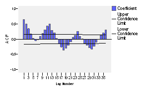
The autocorrelation function (ACF) and the partial autocorrelation (PACF) of the series logarithmically transformed and with a differentiation of order 1 is presented in figures 5 and 6 respectively. The autocorrelation function (ACF) shows significant peaks at lags of 12, 24 and 36, this significance is present at lags of 12 and 24 of the partial autocorrelation function too, but a dwindling is not observed in any of the two, so it is obvious the lack of stationarity.
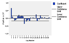
Due to the results mentioned above, the sequence plot and correlograms (see figures 7, 8 and 9 respectively) for the series logarithmically transformed and differentiated in its seasonal and non-seasonal parts are built.

As it can be observed in the figure 7, the sequence plot shows how all observations move around the zero value, so it can be concluded that the series is stationary.
When analyzing the simple and partial autocorrelogram functions in figures 8 and 9 respectively, it is evident that the they fulfill the conditions for the presence of stationarity.
As it can be noticed, the coefficients of both autocorrelation functions have nonzero coefficients in multiples (12, 24, 36) of the seasonal period. Moreover, the autocorrelation function (ACF) takes a sinusoidal shape and decays quickly, which completes its cycle by spinning on the axis and for a quantity of lags equals to the seasonal period.
According to what it has been mentioned previously, the regular part of the series is integrated by zero (o) order = I(0) and the seasonal part is integrated by a first order = I(1).
So, it is necessary to identify the autoregressive part of the series, for which it is analyzed the two correlograms, numbered as 7 and 8; observing that their coefficients do not make abruptly null, so their structure adjust to the following models: ARIMA (1,0,1)x(1,1,1)12, or ARIMA (1,0,1)x(0,1,1)12, or ARIMA (0,1,1)x(0,1,1)12. Both models are tested according to the assumptions they have to fulfill, and the ARIMA (0,1,1)x(0,1,1)12 is selected. The rest of the models identified are discarded because of the presence of non-significant parameters.
Phase 3: Diagnostic checking
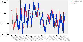
As it can be noticed in the figure 10, the model fits well the data; so, it shows a good agreement between observed values and fit values, indicating that the model has a satisfactory predictive ability. It also does a good job by capturing the seasonality. The dataset covers a period of 12 years and includes 12 seasonal peaks and those values predicted match up well with the 12 annual peaks in observed values. The next step would be to check whether the model fulfill the statistical properties of the error terms (normality assumption, white noise assumption) and the other statistics which should be checked.
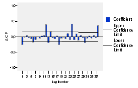
After checking that the model is fit to the data, the analysis of the residuals is necessary, in order to validate the model. One test that should be taken into account is to check whether the residuals are white noise; if they are, the particular fit is accepted, if there is autocorrelation of errors, the model should be specified once again in the tentative model identification stage.
According to the residuals correlation assumption, it has been stated the following hypotheses:
H 0 : the residuals are uncorrelated,
H 1 : the residuals are correlated.
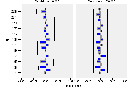
Then, the correlogram of the residuals is built as shown in the figure 11, in which is observed that none of the lags are significant or out of the confidence limit; so, it can be assured that the residuals are a white noise process and that they are uncorrelated, reasons for which the null hypothesis (H 0 ) is accepted.
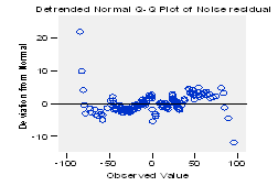
The same way, the normality assumption of the residuals has been stated as follows: H0: the residuals are normally distributed, H1: the residuals are not normally distributed.
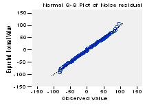
When analyzing the results shown in the figure 12, related to the standard normal probability (Q-Q) plots of the residuals, the null hypothesis (H0) is accepted; observing how all the observations perfectly adjust to the line in the trend Q-Q plot of the noise residuals and how they are randomly distributed in the detrended Q-Q plot of the noise residuals (see figure 13).
When observing the statistics obtained during the validation of the model, the goodness-of-fit is also confirmed with: the stationary R-squared = 0.647, the R-squared = 0.950, MAPE (mean absolute percentage error) = 3.3%, which is equivalent to the uncertainty of the model prediction and considered by Tshepiso Tsoku, et al., (2017), as being very accurate as shown in the table 1; the MaxAPE for the worst scenario of 21%, and a Ljung-Box of 0.262 > 0.05. All these values represent an acceptable amount of uncertainty to assume.
Then, the parameters of the model are presented in the table 3, where it is appreciated that:
As well as the significance of each parameter.
Table 3 - ARIMA Model Parameters.
| Estimate | SE | t | Sig. | ||
|---|---|---|---|---|---|
| Difference | - | 1 | - | - | - |
| MA | Lag 1 | ,510 | ,079 | 6,473 | ,000 |
| Seasonal Difference | - | 1 | - | - | - |
| MA, Seasonal | Lag 1 | ,661 | ,090 | 7,377 | ,000 |
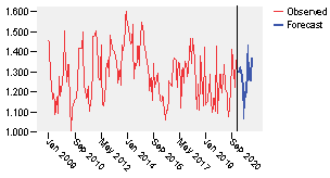
Phase 4: forecasting
The other step is the forecasting of the values to be planned for 2021. The plot of the forecasting results is shown in the figure 14, where the commonalities between what happens in the last length of observed data and the forecasting are visible.
The equation of the model is shown in the expression 12:
The values obtained as part of the forecasting and expressed in blisters are shown in the table 4.
3- Third stage: adjusting of the forecasting
Data obtained from the forecasting process are adjusted to the changes which the morbidity could have experienced.
Table 4 Forecasted values for 2021 expressed in blisters.
| Model | |||||||
|---|---|---|---|---|---|---|---|
| - | Forecast | UCL | LCL | - | Forecast | UCL | LCL |
| Jan 2021 | 1301 | 1438 | 1163 | Jul 2021 | 1202 | 1418 | 987 |
| Feb 2021 | 1299 | 1452 | 1145 | Aug 2021 | 1211 | 1437 | 985 |
| Mar 2021 | 1322 | 1489 | 1154 | Sep 2021 | 1383 | 1619 | 1148 |
| Apr 2021 | 1300 | 1480 | 1119 | Oct 2021 | 1273 | 1518 | 1028 |
| May 2021 | 1247 | 1440 | 1054 | Nov 2021 | 1263 | 1517 | 1009 |
| Jun 2021 | 1135 | 1340 | 931 | Dec 2021 | 1375 | 1638 | 1112 |
Data to adjust the forecasting is obtained from the pharmaceutical technical department. The results of the adjustment are shown in the table 5.
Table 5 - Adjusted Forecasting for 2021 expressed in blisters.
| Model | |||||||
|---|---|---|---|---|---|---|---|
| - | Forecast | UCL | LCL | - | Forecast | UCL | LCL |
| Jan 2021 | 1430 | 1438 | 1340 | Jul 2021 | 1202 | 1418 | 987 |
| Feb 2021 | 1570 | 1492 | 1325 | Aug 2021 | 1211 | 1437 | 985 |
| Mar 2021 | 1420 | 1489 | 1270 | Sep 2021 | 1383 | 1619 | 1148 |
| Apr 2021 | 1400 | 1480 | 1200 | Oct 2021 | 1273 | 1518 | 1028 |
| May 2021 | 1247 | 1440 | 1054 | Nov 2021 | 1263 | 1517 | 1009 |
| Jun 2021 | 1135 | 1340 | 931 | Dec 2021 | 1375 | 1638 | 1112 |
4- Fourth stage: forecasting accuracy
The measurement of the forecasting accuracy will be performed during 2021, to the extent that the actual demand is recorded in each month.
The results obtained in the application of the proposed procedure have a practical implication in the drug inventory management process in pharmaceutical entities. These reflect the need to continue researching in studies related to this topic. The study of the demand is a key factor for the planning process of pharmaceuticals, as well as in responding to patients’ health needs.
Conclusions
The combination of historical data and morbidity in forecasting demands for medications has a direct impact on the accuracy of the planning process of such goods. The procedure designed takes into account this issue.
After applying the four stages of the procedure to one drug, the ARIMA (0,1,1)x(0,1,1)12 model was selected, for this model was the best out of three tested. This selection was made taking into account the results shown in its statistics, the uncorrelated characteristics of its residuals and the capacity of prediction of the model.
The Box-Jenkins methodology have been implemented within the procedure, being part of its second stage. This methodology has been scarcely used in medications inventory forecasting; being demonstrated in this study its applicability in this research area, which supports the planning process of pharmaceuticals.
In future studies, the procedure should be implemented in forecasting the demand of other medications, which will contribute to its further validation.

