Articulo original

Applying Bayesian networks in student dropout data

Aplicación de redes bayesianas en datos de abandono estudiantil

Byron Oviedo Bayas^{1  *} 
http://orcid.org/0000-0002-5366-5917

Jorge Gómez Gómez² 
http://orcid.org/0000-0001-8746-9386

Cristian Zambrano Vega¹ 
http://orcid.org/0000-0001-8568-8024

Evelym Ruth Morán Morán¹ 

¹ Universidad Técnica Estatal de Quevedo. Ecuador.

² Universidad de Córdoba. Colombia.

ABSTRACT

This paper presents a proposal to implement a cluster method that best engages the educational data (socio-economic, academic achievement and dropouts) at the Engineering Faculty of Quevedo State Technical University. The use of graphical probabilistic models in the field of education has been proposed for this research. To complete the student diagnosis, and to predict their behavior as well, an analysis of such Bayesian networks learning models, as PC, K2, and EM optimization was made first. There should be a test for each case where the probability is measured in every model using propagation algorithms. Then, probability logarithm is applied to each case and the results are added in each model to determine the best fit for the proposed. The results of this research will help raise awareness of the various factors affecting students’ performance. Besides, this will allow institutional authorities to identify mechanisms for improving retention index and students’ academic achievement, what serves the improvement of quality indicators in face of institutional and program evaluation and accreditation processes.

Keywords: Bayesian networks; K2; PC; EM; academic performance

RESUMEN

Este artículo presenta una propuesta para implementar un método de conglomerados que mejor involucre los datos educativos (socioeconómicos, rendimiento académico y deserción) en la Facultad de Ingeniería de la Universidad Técnica del Estado de Quevedo. Para esta investigación se ha propuesto el uso de modelos gráficos probabilísticos en el campo de la educación. Para completar el diagnóstico de los estudiantes, y también para predecir su comportamiento, primero se realizó un análisis de modelos de aprendizaje de redes bayesianas, como la optimización de PC, K2 y EM. Debe haber una prueba para cada caso donde la probabilidad se mide en cada modelo usando algoritmos de propagación. Luego, se aplica el logaritmo de probabilidad a cada caso y los resultados se suman en cada modelo para determinar el mejor ajuste para el modelo propuesto. Los resultados de esta investigación ayudarán a crear conciencia sobre los diversos factores que afectan el desempeño de los estudiantes. Además, esto permitirá a las autoridades institucionales identificar mecanismos para mejorar el índice de retención y rendimiento académico de los estudiantes, que sirva para mejorar los indicadores de calidad de cara a los procesos de evaluación y acreditación institucional y de programas.

Palabras clave: Redes bayesianas; K2; PC; EM; rendimiento académico

Introduction

Bayesian networks are known in the existing literature under such other names as causal networks or causal probabilistic networks, networks of beliefs, probabilistic systems, expert Bayesian systems, or also as diagrams of influence Bayesian networks are statistical methods representing uncertainty through conditional independence relationships established among them (^{Edwards, 1998}). This type of networks codifies the uncertainty associated to each variable through probabilities (^{Fernández, 2004}). It is said that a Bayesian network is a set of variables, a graphic structure connected to these variables and a set of probability distributions.

A Bayesian network is a directed acyclic graph, in which each nodule represents a variable and each arc a probabilistic dependency where each variable conditional probability is specified according to its parents; the variable to which the arc is directed is dependent on the one in its origin. Network structure or topology provides information about probabilistic dependencies between variables and also about conditional independencies of a given variable (or set of variables) given another or other variables. Such independences simplify knowledge representation (less parameters) and reasoning (spread of probabilities)

Obtaining a Bayesian network from data is a learning process divided in two stages: structural learning and parametric learning (^{Pearl, 2011}). The first consists in obtaining the structure of the Bayesian network, i.e. dependence and independence relationships between the variables involved. The second stage aims at obtaining probabilities a priori and required conditionings from a given structure.

This paper makes reference to the research on the use of graphic probabilistic models in the field of education for diagnosing students and for determining the drop out problem in universities, as a continuity to previous research. Magaña Echavarria analyzes this problem using cluster and grouping individuals or objects in sets according to their similarities, maximizing object homogeneity within the clusters while maximizing heterogeneity among aggregates (^{Magaña, et al., 2006}). Other studies to predict the probability of student dropout have been carried out using data mining techniques to achieve the objective. Among them ( ^{García Martínez, et al. (2010}), whos made a paper based on the use of knowledge, on discovery rules, and on TDIDT (Top Down Induction of Decision Trees) approach using the academic management data provided by consortium SIU from Argentina, (integrated by 33 universities). This permits to carry out an interesting analysis to find the rules of behaviour containing absentee variables. This paper focuses on applications of probability models in higher education.

This paper is developed on a knowledge basis of 773 students registered for the 2012- 2013 academic year in the Faculty of Engineering Sciences of Quevedo State Technical University. The paper is structured as follows: In section 1 the main aspects of Bayesian learning are described. In section 2 reference is made to Bayesian learning. Next, in section 3 a study of the parameters for the proposal is made together with an experimental comparative analysis with the results obtained using other algorithms mentioned in the state of arts analysis. Section 4 presents conclusions and recommendations.

If we have a set of variables denoted X={X1, X2, .., Xn} where each variable Xi takes values within a finite set Ωxi ; then we use xi to express one of the values of X_i , x_i ∈ Ωxi. Now if we have a set of indexes denoted as I, we symbolize xi, i∈I. We will notice that the set of all the indexes N= {1, 2, .., n} and ΩI represents Ωxi elements and they are called X_i configurations (settings) which will be represented as x or xI.

Bayesian Network its a directed acyclic graph representing a set of randomised variables and their conditionings (see Fig, 1) where Xi is a random happening represented by each node (set of variables) and the topology of graphic shows independence relationship between variables according to d- isolation criterium (^{Pearl, 1988}; ^{Cheeseman, et al., 1993}). Each node X_i has a conditional probability distribution pi(X_i|Π(X_i)) for this variable , given their parents. So a bayesian network determines a unique distribution and joint probability (E1):

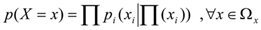
(E1)

Fig. 1 - Example of Bayesian Networks.  

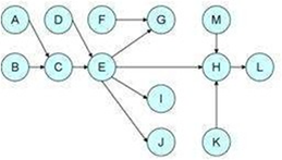
Automatic learning is divided into supervised (Figure 1) and unsupervised learning. In supervised learning the focus of attention is the exact forecast, while the objective in unsupervised learning is to find compact description of data. In both learnings the interest lies on the method fully generalizing the new data. In this sense difference is established between the data used for training a model and the data used to test the functioning of the model being formed.

Definition of Supervised Learning: Given a set of data D= {(xn, cn), n = 1, ..., N}; where (x_n, c_n) is the set of observations where we have a special variable C considered the class, it is necessary to learn the relation between input x and output, so that when a new input x* appears, the predicted output is exact

Pair (x*, c*) is not in D, but it is assumed to be generated by the same unknown process that generated D. To explicitly specify what this means a loose function L(cpred, ctrue) is defined or, on the contrary a utility function U=-L is defined. The utility here is usually 0 or 1, L(cpred, ctrue)=1 si (cpred ≠ ctrue); L(cpred, ctrue)=0 si (cpred = ctrue). In this type of learning what matters is p (y | x, D). conditional distribution. The output is also called “label”, particularly when speaking about classification. Term classification denotes that the label is discrete, i.e. consists in a finite number of values

Bayesian Classifiers: any Bayesian network can be used to make a classification just by distinguishing the variable of interest in the problem as the class variable and then applying any propagation algorithm with the new evidences and a decision rule, so that the results are a value for the class (^{Murphy, 2012}). To determine the best classifier or the one which best suits our study, the one obtaining the highest rate of classification successes will be identified, what would allow to approach the best Bayesian representation of the database.

The simplest and most commonly used graphic probabilistic model for supervised classification is Naive Bayes, which is based in two assumptions: First: each attribute is conditionally independent from the attributes given the class and, second: all the attributes influence the class. BN has demonstrated being comparable, in terms of classification accuracy in different domains of many, more complex algorithms, such as neuronal networks and decision trees (^{Webb & Pazzani, 1988}). The algorithm uses the training data to estimate the required probability values.

Definition of unsupervised learning: given a set of data D = {xn , n = 1, ..., N} the objective is to find an accurate decision of data. It is used to measure the accuracy of the description. In this type of learning there isn’t a special prediction variable, from the probabilistic viewpoint, the interest lies on p (x) distribution modeling. Model probability to generate data is a popular measure of description accuracy (^{Michalski, 1986}).

Fig. 2 - Naives Bayes classifier. 

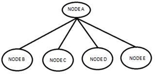
Unsupervised learning are sets of observations (Figure 2) without associated classes, whose aim is to detect regularities in data of any kind. Unlike supervised learning, this kind of learning does not approach input objects as a set of random variables. They are widely used for data compression and grouping.

Fig. 3 - Grouping with unsupervised learning. 

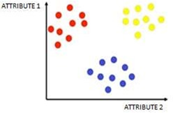
Some unsupervised learning techniques are clustering (Figure 3) (objects are grouped in regions, where similarity is high), visualizing (it allows observing instance space in a lesser dimension space), reducing dimensionality (input data are grouped in subspaces of a lower dimension than the initial), extracting characteristics (they build new attributes from multiple original attributes.

This paper will use clustering to discover the structure of input data looking for groupings among variables and case groups, so that each group is homogeneous and different from the others. There are various clustering methods, among the most known of which we can mention hierarchical (data are grouped in treelike structures), non hierarchical (partitions are generated only at one level), parametric (it assumes that conditional densities of the groupings have a certain known parametric shape and focuses only on estimating the parameters), non parametric (they don’t have any concern about the way in which objects are grouped.

It is common to find variables that, being important to the explanation of the studied phenomenon, were not studied and it can also be noticed some non easily perceived influence on data, and this makes possible to postulate the existence of some hidden variables, responsible for explaining this abnormal production of data (^{Rechy-Ramírez, et al., 2011}).

Each of these algorithms uses an evaluation function together with a method measuring the goodness of each explored structure within the total set of structures. During the exploration process, the evaluation function is applied to assess the adjustment of each candidate structure to the data. Each of the algorithms is characterized by the evaluation function and the search method used. Each of the algorithms uses, for the evaluation function, a metrics not specialized in classifying, commonly known in Bayesian network learning as BIC (^{Schwarz, 1978}), BDEu (^{Heckerman, et al., 2007}), K2 (^{Cooper & Herskovits, 1992}). For efficiency purposes the metric used should be detachable, so that we have only the part modified by the operator and not the whole graph. K2 metric for a G network and a D database is the following:

As we wish to identify the network, which best adapts to the data, we have analyzed various algorithms of Bayesian learning PC algorithm: It is one of the algorithms used (E2):

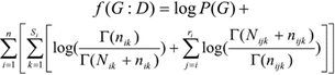
(E2)

Where: N_ijk is the frequency of the settings for Bayesian learning. This algorithm is based on independence tests among variables I(X_i, X_j | A),where A is a subset of variables assumed to have enough data and statistical tests have no mistakes. PC algorithm begins with a full non directed graph to be reduced lately step by step. First, the edges joining two nodes which verify a zero order conditional independence are eliminated, then those of order one, and subsequently, the rest. The set of nodes candidate to form the separating set (the set being conditioned) is the one of the nodes adjacent to any of the nodes intended to be separated. In this paper we used the new PC implementation made in program Elvira, with 0.05 significance level. PC calculates based on independence instead of on score optimization. The algorithms based on score+search functions intend to have a graph better modelling input data, according to a specific found in D database of x_i ; n is the number of variables , taking their j-th value and their parents in G taking their K-.th setting; s_i is the number of possible settings of the parents’ set; ri is the number of values that variable x_i can take;(3) (Γ is function Gamma)

BIC metric is defined as follows (E3):

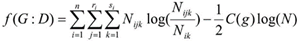
(E3)

Where: N is the number of database registers; C(G) is a complexity measure for G network, defined as (E4):

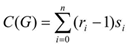
(E4)

BDEu metrics depends on only one parameter, the sample size α and is defined as follows (E5).

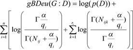
(E5)

Algorithm K2: It is based on the search and optimization of a new Bayesian metrics. K2 makes a voracious and very effective search to find a good quality network in an acceptable time (^{Dempster, et al., 1977}). K2 is a heuristic codicious algorithm basing on the optimization of a measure. That measure is used to explore, through a hill ascension algorithm, the search space formed by all the networks containing the database variables. This algorithm establishes an order among the variables.

To define the network with this algorithm we should follow three important steps:

• An initial graph without arcs should be present.

• An arc to be added to the graph is selected.

• We calculate the score of the new network with a new arc at each step.

• The arc with the highest score is chosen.

• If the new arc increases the probability of a new network, it is added and step 2 is taken, otherwise, that would be the network.

• An order of variables is supposed to exist. EM algorithm (Expectation Maximization) (^{Sierra, 2006}) is a method to find the estimator of maximum likelihood for the parameters of a probability distribution. This algorithm is very useful when part of the information is hidden. To find these optimum parameters two steps should be followed: first (Expectation) to calculate the expectation of likelihood with respect to the information known and some proposed parameters, then (Maximization) to maximize with respect to the parameters; these two steps are repeated until convergence is achieved (^{Oviedo, et al., 2016}).

Materials and methods

In this section an experimental study has been prepared to carry out the analysis of the data using RB techniques presented in the software. Below the phases carried out for the analysis are presented.

Analysis of data, identification of attributes and imputation.

Table 1 - Description of the data file. 

Variable	Description
A	Career (Program)
B	Year
D	Disabled
E	Education cost
F	Lives apart from family
G	Type of family housing
H	Home owner
I	Cable tv service
J	Credit card service
K	Internet access service
L	Basic services
M	Private transportation services
N	Cell phone plan service
O	Own car services
P	Own car comes services
Q	Currently working

Table 1 identifies the variables studied. Here we can find socioeconomic variables represented with letters from D to Q and here you can also visualize variables describing or identifying the studies in which they were represented with letters A and B, which can be visualized in table 2, and finally variables representing academic achievement represented with letters R and S.

Table 2 - Careers(programs) of science engineering faculty. 

Codex	Career (Program)
FI024	Systems Engineering
FI025	Graphic Design Engineering
FI026	Mechanical Engineering
FI027	Industrial Engineering
FI028	telematics Engineering
FI029	Electrical Engineering
FI030	I Agroindustrial Engineering
FI031	Industrial Safety Engineering.

The variables state of approval and student dropout were encrypted with values 1 and 0 to identify the study cases.

Discretization of variables

Elvira provides a great number of discretization methods. Among the most outstanding variables are: Discretization for the same width, Addition of different squares, Mono Technical contrast without supervision. K-media Discretization. The continuous variable selection methods search for obtaining a new set of discrete variables from the original continuous set for classification with the objective of problem simplification, higher learning speed, greater interpretability and an increase of success percentage.

In this paper the discretization process was carried out manually through expert criterion. Table 3 shows the discretized values of each of the variables.

Table 3 - Discretized variables. 

Attribute	Discretization
Disabled	YES= 1; NO=0
Education cost	X<200=0; 200>X<800=1; X>800=2
lives apart from family	YES= 1; NO=0
Type of housing FAMILY	WATER AVERAGE = 0; HOUSING/VILLA = 1 DEPARTMENT=2
Tipo vivienda FAMILIA	TENANT ROOMS= 3; OTHER= 4; RANCH= 5
Home owner FAMILY	FATHER AND MOTHER =0; FATHER = 1; MOTHER = 2; ANOTHER RELATIVE =3; OTHER=4
tv cable service	SI= 1; NO=0
Credit card service	SI= 1; NO=0
Internet access service	SI= 1; NO=0
Basic services	SI= 1; NO=0
Private transportation service	SI= 1; NO=0
Cellphone plan	SI= 1; NO=0
Own vehicle service	SI= 1; NO=0
Currently working	SI= 1; NO=0
Passes the test	SI= 1; NO=0
Drops out	SI= 1; NO=0

Results and discussion

At the beginning of the different tests and experiments, the Cluster technique was used with the objective of obtaining classifications (clustering’s) of the cases sharing the same characteristics i.e. those which are similar, being the different groups among them as different as possible.

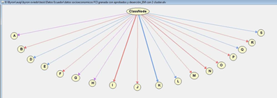
As we want our network to learn, we focus on automatic learning, choose the classifier with Laplace selection, and do the processing taking into consideration the variables shown in Table 1. Figure 4 shows the Bayesian network generated from a Naive Bayes classifier, which through a supervised prediction builds up this model allowing us to predict the probability of possible results.

Fig. 4 - Naives Bayes classifier for study data. 

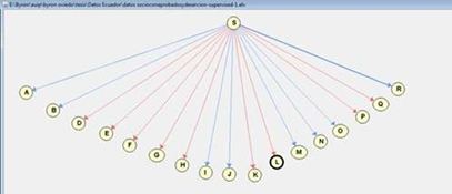
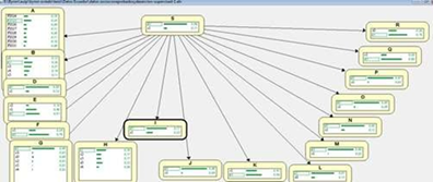
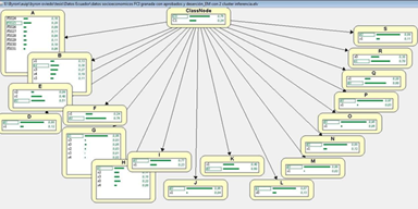
Fig. 5 - Bayesian Network from the data where the network node of influence is marked (inference mode). 

Figure 5 shows the same network, but in the inference mode, where the probability of each value is shown through a bar with a length proportional to probability and through a number. Since no findings have been introduced, probabilities appear a priori.

Below a study to find the groups of closely connected variables by means of algorithms and parameters shown in Table 4 is presented.

Table 4 - Methods used. 

Metho d	Classificati on	Clas- mét	Clus- pad	Estimation
K2	Factorization	BDE	5	LAPLACE
PC	Factorization	BIC	5	LAPLACE
EM	Unsupervized	CBN	2	LAPLACE

As shown in Figure 6 Elvira software has provided three parent nodes which are: career (program), family type of housing, and if the student is disabled or not, each of them being related to other variables. It can be noticed that variable Passed(R) relates to variable Dropout (S) and that both Career (A) and Course (B) indirectly influence Dropout ( S). On the other side, the socioeconomic variables, very closely related with one another, but without any influence on the student passing or dropout are located.

Fig. 6 - Bayesian network trying K2, maximum 5 parents, BIC Bayesian estimation. 

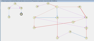
According to Figure 7, once working with 773 cases (students legally registered during 2012- 2013 academic year), it is possible to determine the strong influence of those who have their own car and come to the university using this means of transportation. Likewise, figure 7 shows that having a private means of transportation usually implies having cell phone plan service and cable tv.

Fig. 7 - Bayesian network trying PC, maximum 5 parents. 

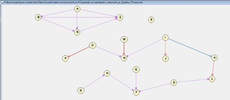
We can identify the way variables get grouped. On one side the program relates to course, pass, and dropout in a manner distant to other groupings. The variable cost is isolated from all the groupings.

It can be easily noticed that the type of relationships do not differ too much from the previously analyzed algorithms (many remain the same), but on the other hand, new groupings are generated, many of them isolated, among the variables not having a relation similar to the one obtained with K2.

Working with two clusters allows obtaining a class node, on which variables depend. This puts into evidence the stronger relationship with the tv cable and the internet services as shown in Figure 8.

Fig. 8 - Bayesian Network trying EM with 2 clusters (edition mode). 

Fig. 9 - Bayesian network trying EM con 2 clusters (inference mode). 

According to Figure 9, the percentage of students who drop out of their university studies can be determined as well as, that the program with the highest dropout index is Graphic Design Engineering with a 28 percent, and the year with the highest dropout incidence is the Second with a 30 percent, followed by the Third with a 27 percent. 30 percent of students do not manage to pass the subjects they are taking, so the majority registers for the second time in the program.

The dropout problem in the programs of the Faculty of Engineering Sciences at Quevedo State Technical University during 2012-2013 academic year is directly tied to the socioeconomic factor. 24 percent of students live apart from their families, 86 percent of the housings are villa-style and 33 percent of house owners are fathers. It is also important to indicate that 77 percent of students do not have cable tv service and only the 4 percent have a credit card. The 40 percent of students can connect to the Internet from homes. On the other hand, only 2 percent of students have private transportation, 12 percent have cell phone plans, the 5 percent have cars, but only the 3 percent comes to the university in self- owned cars. It should be said that 20 percent of these students work, what results in 30 percent student failure and from this 11 percent drop out of university studies and take the failed subject one more time. These data are the result of the convergence such variables as low family income, unemployment, and work - and study incompatibility as the main causes.

This problem is studied in this paper by applying k2, PC, and EM algorithms, which help to group variables as models for finding groups of strongly related variables. The results found can be summarized as follows:

After running k2 algorithm, we have seen that it shows sets of grouped variables, which defined a possible cause of student dropout. Taking as reference the first of these groupings, we can observe that variables Career (A) and Course (B) strongly influence variable Pass (R), in the same way these influence dropout(S). Even talking about the data, we notice that there is 11 percent probability of a student dropping out during the program, due to career wrong selection. It can also be noticed that 30 percent of these students drop out on the second year of the program.

1. PC algorithm with 5 parents and 733 cases, shows a similar grouping of variables, but with different sets of relationships. This algorithm allows to observe that variable A highly influences variables B, S, and R, taking as reference that the greatest number of dropouts comes from one program and is located mainly in its second year.

2. In the case of EM with two clusters, we can determine a relationship between a class variable and the rest of the variables, considering C as the class variable and the rest as children’s nodes.

3. After having applied the referred algorithms, it can be noticed that they had in common the grouping of variables A, B, R, and S in one set of variables, as well as the strong influence of variable A on the rest of the set variables, what makes it a possible direct cause of student dropout.

Conclusions

A student retention or dropout of the university and the successful culmination of studies are influenced by different factors: individual, academic, socioeconomic, and institutional. In this sense, the dropout will continue, in spite of any changes in higher education institutions. Research on this problem allows providing solutions to partially control dropout indexes and retain students in their programs

Results evidence that an impact factor for student dropout is the year they are in, as well as the different socioeconomic factors directly influencing the student’s academic performance.

It is suggested to check the different selection and admission processes of the applicants for Quevedo State Technical University to detect possible dropouts. Besides, it is recommended to implement fellowship programs and economic support for the students who need it, and thus, diminish dropout once it is previously known that economic problems are no longer a barrier to students’ enrollment in a program due to education gratuity.

In a future paper we propose to relate other variables to have a clearer idea of the reasons of student dropout and the passing of courses, as it is the case of working with variables relating to teachers’ staff and to the higher institution education itself. It is indispensable that teachers assume the institutional objectives as their own.

References

Cheeseman, P., Self, M., Kelly, J., Stutz, J., Taylor, W., & Freeman, D. (1993). Autoclass: a bayesian classification system. In Readings in know- ledge acquisition and learning. Morgan Kaufmann Publishers Inc.

Cooper, G., & Herskovits, E. (1992). A bayesian method for the induction of probabilistic net- works from data. Machine learning, 9, 309-347.

Dempster, A. P., Laird, N. M., & Rubin, D. B. (1977). Maximum likelihood from incomplete data via the EM algorithm. Journal of the Royal Statistical Society. Series B (Methodological), 39(1), 1-22.

Edwards, W. (1998). Hailfinder: Tools for and experiences with Bayesian normative modeling. American Psychologist, 53(4), 416-428.

Fernández, E. (2004). Análisis de clasificadores bayesianos. (Trabajo final de especialización). Instituto Tecnológico de Buenos Aires.

García Martínez, R., Kuna, H. D., & Villatoro, F. (2010). Identificación de causales de abandono de estudios universitarios. TE & ET, 5, 39-44.

Heckerman, D., Kadie, C., & Listgarten, J. (2007). Leveraging information across hlaalleles / supertypes improves epitope prediction. Journal of Computational Biology, 14(6), 736-746.

Magaña, M. A., Montesinos, O. A., & Hernández, C. M. (2006). Análisis de la evolución de los resultados obtenidos por los profesores en las evaluaciones esdeped y las realizadas por los estudiantes. Revista de la Educación, 35(4), 29-48.

Michalski, R. S. (1986). Machine learning : An artificial intelligence approach. Morgan Kaufmann.

Murphy, K. P. (2012). Machine learning : a probabilistic perspective. MIT press.

Oviedo, B., Moral, S., & Puris, A. (2016). A hierarchical clustering method: Applications to educational data. Intelligent Data Analysis, 20, 933-951.

Pearl, J. (1988). Probabilistic reasoning in intelligent systems: networks of plausible inference. Morgan Kaufmann.

Pearl, J. (2011). Bayesian networks. Department of Statistics, UCLA.

Rechy-Ramírez, F., Acosta-Mesa, H. G., Mezura-Montes, E., & Cruz-Ramírez, N. (2011). Times series discretization using evolutionary programming. (Ponencia). 10th Mexican International Conference on Artificial Intelligence, MICAI 2011. Puebla, Mexico.

Schwarz, G. (1978). Estimating the dimension of a model. The annals of statistics, 6(2), 461-464.

Sierra Araujo, B. (2006). Aprendizaje automático: conceptos básicos y avanzados. Aspectos prácticos utilizando el software Weka. Pearson Prentice Hall.

Webb, G. I., & Pazzani, G. I. (1988). Adjusted probability naive bayesian induction. In Proceedings of the Eleventh Australian Joint Conference on Artificial Intelligence. Springer- Verlag.

Received: January 08, 2022; Accepted: March 27, 2022

^*Autor para correspondencia. E-mail: [e-mail]

Los autores declaran no tener conflictos de intereses.

Los autores trabajaron en la elaboración total del artículo.