Original article

Time series prediction model for the tourism demand of the Cubanacán Hotel Chain

0000-0003-1974-9209Reinier Fernández López^{1  *}  , 0000-0002-8923-764XLedy Raúl Díaz González¹  , 0000-0002-4885-5337Juan Carlos Alfonso Alemán²  , 0000-0001-9256-2980Olga Barrio Padrón³ 

¹ Universidad de Pinar del Río "Hermanos Saíz Montes de Oca". Facultad de Ciencias Técnicas. Departamento de Matemática. Pinar del Río, Cuba.

² Fondo Cubano de Bienes Culturales. Pinar del Río, Cuba.

³ Delegación Provincial del Ministerio de Turismo. Pinar del Río, Cuba.

ABSTRACT

The tourist demand has a vital influence on the planning and projection of the decision makers in this activity. In this sense, prognosising the tourist demand, thus integrating the productive chains to the rest of the socio-economic activities of the production and service processes, becomes an unavoidable tool. The objective of this work is to elaborate a prognosis model for the tourist demand through the use of techniques of temporary series, which allows predicting the behavior of tourism, sustained in the Box-Jenkins methodology and which supports the process of decision making in Cubanacán Hotel Chain of Pinar del Río, Cuba. It was possible to formulate a rigorous model with the use of statistical-mathematical methods as guiding axes of the research; also, it was modeled the tourist demand until December 2019.

Key words: demand; Box-Jenkins methodology; time series; tourism

Introduction

Deficient planning of tourism implies bad management that, without a doubt, degrades this activity. Destinations around the world benefit when this sector is properly managed, based on adequate planning ^{(Hącia, 2019)}. The integrating effect that covers almost all sectors of the economy makes tourism one of the most diverse industries in the world ^{(Meschede, 2020)}.

Its social effects are innumerable and it can also be seen as an economic activity by defining elements. That is why the tourism sector must be able to understand the demand and how it will be distributed over time ^{(Feng et al., 2019)}.

In that sense, the demand of a destination becomes a very important object of study: to know the characteristics of the travelers, to which segment they belong, the tourist expenditure, the levels of satisfaction, among others. The analysis of the distinctive features of tourism demand leads to the design of actions so that the destination is capable of satisfying the needs and desires of the tourist ^{(Chenguang Wu et al., 2017)}.

Focusing on long-term prognosising (monthly, quarterly, and annual) of relatively large areas (provinces, countries, and regions) allows for the estimation and analysis of future demand for a particular product, component, or service through different prognosising techniques. Prognosising future demand is central to any planning and operational activity, particularly in activities related to logistics and the supply chain.

It is evident the relevance of prognosising to plan the productive system, the supply and the dispatches, so that the supply chain operates correctly. These tools allow for relevant, precise and reliable information to be obtained; therefore, it is necessary for companies to correctly use the most appropriate models and procedures for this purpose ^{(C. Li et al., 2020)}.

At the organizational level, demand prognosising is an essential input for any decision in the different functional areas: sales, production, purchasing, finance and accounting. Prognoses are also necessary in distribution and procurement plans. The importance of a prognosis with a low margin of error is fundamental for efficiency and effectiveness. This has been largely recognized by various authors ^{(Shaowen Li et al., 2018)}.

Framed in this context, there are the antecedents of the first researches regarding the prognosis of tourist demand in Cuba, which are not numerous, but the existing ones contain a high degree of practical and scientific novelty. Such is the case of the prognoses carried out by the Center for Tourism Studies of the University of Havana and by the National Institute of Economic Research of the Ministry of Economy and Planning of Cuba.

Among the most relevant authors that deal with elements on the studies of tourist demand in Cuba, they stand out: Figuerola et al. ⁽²⁰⁰⁵⁾, Rigol Madrazo et al. ⁽²⁰⁰⁹⁾, Josefá Barbosa and Parada Gutiérrez ⁽²⁰¹⁰⁾, Rodríguez Betancourt and Estévez Mártir ⁽²⁰¹²⁾, La Serna Gómez ⁽²⁰¹²⁾, Delgado Castro and Martín Fernández ⁽²⁰¹⁴⁾, González Laucirica and Santa Cruz Rodríguez ⁽²⁰¹⁴⁾ and Díaz Pompa et al. ⁽²⁰²⁰⁾.

In a general way, these researchers propose models that contemplate, as advantages, characteristics of the prognosis of the tourist demand in the short and medium term; they include factors that can modify the prognosis of the demand in the tourist sector, besides segmenting the emitting market; but they do not cover, in an explicit way, the diverse factors that have influenced through time. There are few easy to use mathematical models, based on computer tools; tourism demand prognoses lack projections with different margins of error for a more in-depth analysis or simply mention the tourism demand prognosis as a fundamental tool for decision making without making practical use of it.

Therefore, this research proposes as an objective: to elaborate a long-term prognosis model for tourist demand, through the application of Box-Jenkins methodology, which allows characterizing the tourist evolution in this strategic sector for Cuban economy and projecting prognoses with different levels of reliability.

Materials and methods

Documentary analysis and scientific observation are used to characterize the current situation of tourist demand in Pinar del Rio, Cuba. There are used statistical-mathematical methods and tools such as the Box-Jenkins methodology ^{(Box et al., 1970)}. There were used the soft wares R 3.6.3 and R Studio 1.2.5033 for the processing of data and available information. Theoretical methods were also used to review the development of the current tourism management processes in Pinar del Río. For the analysis, the series number of monthly tourists between January 2006 and December 2018 was used.

The prognosis begins with the identification of the Autoregressive Mobile Media Integration Process, using the auto-arima functions of the R software. With the estimated parameters, the model is formed and validated through the analysis of the residues. The residues must be unrelated so that the model is suitable. This is what is known as the Box-Jenkins methodology ^{(Petrevska, 2017)}.

Integrated Mobile Media Self-Regressive Model

ARIMA is recognized as one of the most important statistical prediction models in time series research and was created by Box and Jenkins in 1970. It marked the beginning of a new generation of prognosising tools, popularly known as Box-Jenkins methodology, but technically known as ARIMA methodology.

It is composed of two models, the Autoregressive (AR) and the Mobile Sock (MA). It has specific parameters for the time series: the p and q parameters, which represent the order of the AR and the order of the MA, respectively. A parameter d is added to represent the number of differences ^{(Shuyu Li et al., 2018)}.

The AR model is written as: y _t = c + a ₁ y _t-1 + … + a _p y _t-p +u _t , donde a ₁ ,a ₂ ,a ₃ ,…,a _p are the parameters of the AR, c is a constant, p is the order of the AR, and u _t is the white noise. Continuously the model MA can be written as: y _t = μ + u _t + m ₁ u _t-1 + … + m _q u _t-q , where m ₁ ,m ₂ ,m ₃ ,…,m _q are the parameters of MA, u _t ,u _t-1 ,…,u _t-q are the terms of the white noise and μ is what is expected from y _t . Integrating these models to obtain the ARIMA model, we have the following expression: y _t = c + a ₁ y _t-1 + … + a _p y _t-p + u _t + μ + u _t + m ₁ u _t-1 + … + m _q u _t-q , where p and q are the terms of the autoregressive and moving average process respectively.

Integrated Autoregressive Seasonal Mobile Media

The Integrated Self-Regressive Seasonal Moving Average Process (SARIMA) is an extension of ARIMA in case the stationary series presents the seasonal component, which includes new terms for order 12 differentiation ^{(Bakar & Rosbi, 2017)}.

The seasonal ARIMA models (P, D, Q) complement the general non-seasonal ARIMA model (p, d, q), developed to capture the quarterly or half-yearly seasonal patterns present in the time series ^{(Box et al., 1970)}. The combination of non-seasonal ARIMA (p, d, q) models with seasonal ARIMA (P, D, Q) leads to the SARIMA (p, d, q)×(P, D, Q) model, also known as multiplicative ARIMA ^{(López et al., 2017)}. In aggregate form, its general representation is: where: d is the number of regular differences, D is the number of seasonal differences, s is the seasonal amplitude, α optimal constant, q is the number of components of moving averages, Q is the number of components of seasonal moving averages, θq are the coefficients of moving averages, Θ _Q are the coefficients of seasonal moving averages, p is the number of autoregressive components, P is the number of seasonal autoregressive components, Ø _p are the coefficients of autoregressive processes, Φ _p are the coefficients of seasonal autoregressive processes.

Autocorrelation function

The autocorrelation function (ACF) is a very useful tool in identifying the order of an MA model. The ACF of an MA_(q) is cancelled after the q delay, i.e. ρ _k ≈ 0 para k > q, then the process can be modeled using a moving average procedure of order q, MA_(q). The ACF represents graphically the correlation values for k time delays ^{(Petrevska, 2017)}.

Given the stationary assumption, where var(y _t ) = var(y _t-1 ) the autocorrelation function is called the partial autocorrelation function (PACF), it represents in the graph the values for a k lag and is implemented to select the order of the AR process. This PACF is built from the following expression: .

Both are used for residue analysis and to check whether the model is suitable or not.

Results and discussion

To fulfill the objective, a univariate analysis of time series was applied, in order to observe the behavior of the series of tourist demand in the Cubanacán Hotel Chain, in the period between January 2006 and December 2018. It should be noted that a time series is composed of trend, cyclical fluctuation, seasonal variation and irregular movements.

When making the graphic representation of the series, it can be classified as stationary, since it oscillates around the historical average value of 4364 tourists as can be seen in figure 1. The Dickey-Fuller test, increased by R, confirms this classification, with a probability value of 0.02647, not exceeding the significance level of 0.05. It should be remembered that this has as an alternate hypothesis that the time series is stationary.

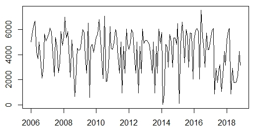Source: R, version 3.6.3

Fig. 1 Time series of the monthly tourist demand (Cubanacán Hotel Chain, 2006-2018) 

By breaking down the time series for trend and seasonality analysis, a graph containing each component of the series, obtained by the moving average method, is presented. Figure 2 shows the observed values, the seasonal component, the trend and the residuals.

Three important fluctuations are also observed: the first begins in 2008 due to the world economic crisis and the scourge of hurricanes Gustav and Ike; the second is evident as of 2013, when the world panicked over the pandemic outbreak of Ebola disease and the third, after 2015, due to the opening of Cuba-United States relations; however, they show a decrease as of 2017 as a result of the decline in these relations.

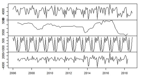Source: R, version 3.6.3

Fig. 2 Method of decomposition by moving averages additive model for the tourism demand time series (Cubanacán Hotel Chain) 

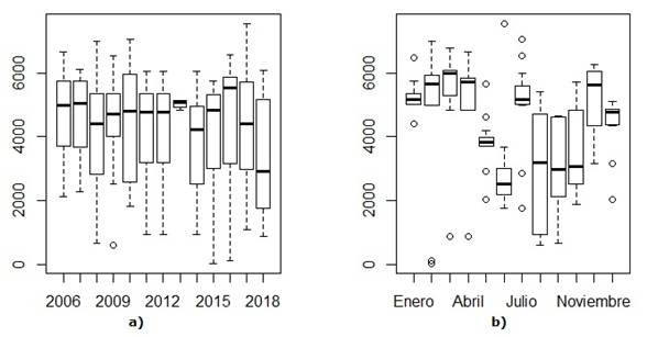
In the box graphs, you can see that the years with the highest peaks were 2006, 2007, 2013 and 2016. In 2013, the highest number of visitors occurred with a low variability and the decrease from 2017 is corroborated (Fig. 3a).

Source: R, version 3.6.3

Fig. 3 Box graphs of tourist demand by year and month (Cubanacán Hotel Chain) 

If the series is described by months, the seasons that predominate in the hotel chain can be observed: high season and low season. The high season is conceived from the arrival of the months of low temperatures in the northern hemisphere (from November to April) and the low season, the warmest months (from May to October). From the graph in figure 3b, it can be seen that the months with the most stability for tourism are January and May. This is not the case for the months from August to November.

Table 1 shows the average tourist demand by year and by month. It allows us to determine the years and months of highest and lowest demand.

Table 1 Average for the tourist demand per year and per month 

Month	Average		Year	Average	Year	Average
Ene	5171		2006	4699	2018	3456
Feb	4779		2007	4644
Mar	5506		2008	4121
Abr	4950		2009	4419
May	3778		2010	4448
Jun	2902		2011	4287
Jul	5061		2012	4287
Ago	2870		2013	5023
Sep	2936		2014	3798
Oct	3616		2015	4013
Nov	5177		2016	4566
Dic	4383		2017	4292

Source: Own elaboration

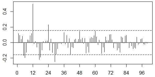
The correlogram of the series of tourist demand in the Cubanacán Hotel Chain, shown in figure 4, allows us to verify that there is a predominance of the seasonal component, evidenced by the presence of a relative maximum for delay 12; in addition to the presence of the trend component, but to a lesser degree, as the values of the autocorrelation function go from positive to negative.

Source: R, version 3.6.3

Fig. 4 Graph of the autocorrelation function for the tourism demand time series (Cubanacán Hotel Chain) 

When detecting these elements, based on the characteristics of the series, the most recommended option is to use SARIMA models. It will be necessary to make a differentiation of order twelve to eliminate the seasonality and thus achieve a purely stationary series prior to the application of the model.

For the selection of the most suitable model, R's auto-arima function was used. From known predictability criteria, i.e., the Akaike Information criterion (AIC), the Corrected Akaike Information criterion (AICc) and the Bayesian Information criterion (BIC). In addition, accuracy measures such as Mean Percentage Error (MPE), Mean Absolute Percentage Error (MAPE) and Mean Absolute Scale Error (MASE) are used. Table 2 shows the results obtained through the software.

Table 2 SARIMA models for the tourist demand time series 

ARIMA tourist demand series (0.0.0) (1.0.0) [12]
Coefficients	Sar1	Average
	0.5412	4217.399
s. e	0.0683	226.816
AIC=2697.39	AICc=2697.55	BIC=2706.52
MPE=-138.9312	MAPE=157.0537	MASE=1.064214

Source: Own elaboration

The most suitable model that minimizes all dispersion measures is a model with an order twelve and order one differentiation in the autoregressive part of the seasonality, that is, a SARIMA model (0, 0, 0) (1, 0, 0), with model equation .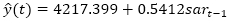

To validate the model, the Ljung-Box-Pierce contrast, also known as the portmanteau test, is performed. The null hypothesis is that the first autocorrelations are null. The result, with a probability value equal to 0.1894, implies that the correlations are statistically equal to zero and, therefore, it can be assumed that the residuals behave as white noise.

This means that the standardized waste varies around the neutral, without trend, with constant variance and no outliers. Approximately 95% of the standardized residuals should be between -2 and 2 standard deviations.

The prognosis of the monthly tourist demand of the Cubanacán Hotel Chain for the year 2019 is shown in the R output of table 3. In this, the prognosis is observed through intervals for 80 and 95% confidence.

Table 3 Prognosis of the tourist demand for 2019 

Month	Year	Prognosis	Inf 80	Sup 80	Inf 95	Sup 95
Ene	2019	4740.0	2924.5	6555.0	1963.4	7516.5
Feb	2019	5141.6	3326.1	6957.0	2365.0	7918.1
Mar	2019	5232.5	3417.0	7048.0	2456.0	8009.0
Abr	2019	2406.1	590.7	4221.6	-370.3	5182.7
May	2019	3515.7	1700.2	5331.2	739.2	6292.2
Jun	2019	2880.8	1065.3	4696.3	104.3	5657.3
Jul	2019	2880.8	1065.3	4696.3	104.3	5657.3
Ago	2019	2902.5	1087.0	4717.9	125.9	5679.0
Sep	2019	3203.4	1387.9	5018.9	426.9	5979.9
Oct	2019	4230.7	2415.2	6046.1	1454.1	7007.2
Nov	2019	3644.0	1828.5	5459.4	867.4	6420.5
Dic	2019	3907.0	1842.7	5971.3	749.9	7064.1

Source: Own elaboration

By means of the plot function of R, it is possible to obtain the graphical representation of the series tourist demand, with its prognosis for the next year as it can be observed in figure 5.

Source: R, version 3.6.3

Fig. 5 Tourism demand prognosis (Cubanacán Hotel Chain, year 2019) 

With the Box-Jenkins methodology, the mathematical model of temporal series was obtained, which made it possible to model the tourist demand in the Cubanacán Hotel Chain for the year 2019. The prognosis of the demand is pertinent, even if the data referred to the study about what has passed from 2020 are added. Obviously, the situation of the pandemic associated with the COVID-19 will introduce heterogeneous mechanisms, but that would ratify other external processes that cannot be ignored.

In the temporal analysis of the series, it is observed the effect of the world economic crisis and the passage of hurricanes Gustav and Ike through Cuban West, it is clearly evidenced the negative impact in the descriptive analysis of the temporal series in question for Cubanacán Hotel Chain. The beneficial influence of the rapprochement in terms of diplomatic relations between Cuba and the United States during the period of the presidency of Barack Obama is also considerable.

Therefore, the mathematical models of time series have to be present for a planning of the economic activity, so that the process of projection and decision making of the organizations is guaranteed. Its effectiveness and ease of use has been proven after creating a friendly methodology for the use of decision-makers, which although it contemplates all the empirical and statistical-mathematical methods used, with the appropriate scientific rigor, it can also allow hotel chains to reach a prognosis that guarantees an interrelationship with their entire local and international environment.

Referencias bibliográficas

Bakar, N. A., & Rosbi, S. (2017). Data Clustering using Autoregressive Integrated Moving Average (ARIMA) model for Islamic Country Currency: An Econometrics method for Islamic Financial Engineering. The International Journal of Engineering and Science (IJES), 6(6), 22-31. https://doi.org/10.9790/1813-0606022231

Box, G. E. P., Jenkins, G. M., & Reinsel, G. C. (1970). Time Series Analysis: Forecasting and Control. John Wiley & Sons, Inc. https://books.google.com.cu/books/about/Time_Series_Analysis.html?id=rNt5CgAAQBAJ

Chenguang Wu, D., Song, H., & Shen, S. (2017). New developments in tourism and hotel demand modeling and forecasting. International Journal of Contemporary Hospitality Management, 29(1), 507-529. https://doi.org/10.1108/IJCHM-05-2015-0249

Delgado Castro, A., & Martín Fernández, R. (2014). Pronóstico de la demanda turística hacia Cuba considerando el impacto del cambio climático. Revista Caribeña de Ciencias Sociales. https://www.eumed.net/rev/caribe/2014/08/pronostico-demanda-turistica.html

Díaz Pompa, F., Leyva Fernández, L. de la C., Ortiz Pérez, O. L., & Sierra Mulet, Y. (2020). El turismo rural sostenible en Holguín. Estudio prospectivo panorama 2030. El Periplo Sustentable, (38), 174-193. https://doi.org/10.36677/elperiplo.v0i38.9265

Feng, Y., Li, G., Sun, X., & Li, J. (2019). Forecasting the number of inbound tourists with Google Trends. Procedia Computer Science, 162, 628-633. https://doi.org/10.1016/j.procs.2019.12.032

Figuerola, M., Chirivella, M., & Quintana, R. (2005). Efectos y futuro del turismo en la economía cubana. Centro de Estudios de Economía y Planificación. https://isbn.cloud/9789597166115/efectos-y-futuro-del-turismo-en-la-economia-cubana/

González Laucirica, Á. M., & Santa Cruz Rodríguez, D. (2014). Turismo senior: Análisis del comportamiento de las edades de los clientes que visitan el hotel X. Varadero, Cuba. RES NON VERBA, 4(1), 20-25. http://biblio.ecotec.edu.ec/revista/edicion5/TURISMO%20SENIOR.pdf

Hącia, E. (2019). The role of tourism in the development of the city. Transportation Research Procedia, 39, 104-111. https://doi.org/10.1016/j.trpro.2019.06.012

Josefá Barbosa, A., & Parada Gutiérrez, O. (2010). Propuesta de un procedimiento para el análisis de la demanda turística. TURyDES, 3(7). https://www.eumed.net/rev/turydes/07/bg.htm

La Serna Gómez, A. (2012). El pronóstico de la demanda turística incluyendo variables mercadológicas. TURyDES, 5(12). https://www.eumed.net/rev/turydes/12/asg.html

Li, C., Ge, P., Liu, Z., & Zheng, W. (2020). Forecasting tourist arrivals using denoising and potential factors. Annals of Tourism Research, 83. https://doi.org/10.1016/j.annals.2020.102943

Li, Shaowen, Chen, T., Wang, L., & Ming, C. (2018). Effective tourist volume forecasting supported by PCA and improved BPNN using Baidu index. Tourism Management, 68, 116-126. https://doi.org/10.1016/j.tourman.2018.03.006

Li, Shuyu, Yang, X., & Li, R. (2018). Forecasting China's Coal Power Installed Capacity: A Comparison of MGM, ARIMA, GM-ARIMA, and NMGM Models. Sustainability, 10(2), 506. https://doi.org/10.3390/su10020506

López, A. M., Flores, M. A., & Sánchez, J. I. (2017). Modelos de series temporales aplicados a la predicción del tráfico aeroportuario español de pasajeros: Un enfoque agregado y desagregado. Estudios de Economía Aplicada, 35(2), 395-418. https://doi.org/10.25115/eea.v35i2.2478

Meschede, H. (2020). Analysis on the demand response potential in hotels with varying probabilistic influencing time-series for the Canary Islands. Renewable Energy, 160, 1480-1491. https://doi.org/10.1016/j.renene.2020.06.024

Petrevska, B. (2017). Predicting tourism demand by A.R.I.M.A. models. Economic Research-Ekonomska Istraživanja, 30(1), 939-950. https://doi.org/10.1080/1331677X.2017.1314822

Rigol Madrazo, L. M., Pérez Campdesuñer, R., Noda Hernández, M. E., & González Ferrer, J. (2009). Modelo y procedimiento para la gestión de la demanda turística. Ciencias Holguín, 15(3), 1-12. http://www.ciencias.holguin.cu/index.php/cienciasholguin/article/view/496

Rodríguez Betancourt, R., & Estévez Mártir, M. (2012). Aplicación de la matemática borrosa para la determinación del presupuesto en instalaciones turísticas. Ciencia en su PC, (1), 94-106. https://www.redalyc.org/articulo.oa?id=181324066008

Received: June 25, 2020; Accepted: December 02, 2020

^*Autor para correspondencia. Correo electrónico: [e-mail]

Los autores declaran no tener conflictos de intereses.

Los autores han participado en la redacción del trabajo y análisis de los documentos.