Original article

Analysis of costs and financial evaluation as a tool for decision making in forest harvesting

0000-0003-2285-7227José Luis Martínez Cantón^{1  *}  , 0000-0001-7627-0152Daniel Alberto Álvarez Lazo²  , 0000-0002-7846-2518Fidel Cándano Acosta³  , 0000-0003-0811-7839Raúl Ricardo Fernández Concepción¹  , 0000-0003-4179-1307Arnaldo Díaz Acosta¹ 

¹Banco Financiero Internacional, Pinar del Rio. Cuba

²Universidad de Pinar del Río "Hermanos Saíz Montes de Oca". Pinar del Río, Cuba.

³Universidad Federal de Mato Grosso, Brasil.

ABSTRACT

The economic efficiency of the harvesting system depends on several factors such as geomorphological and climatic conditions of the felling areas, characteristics of the future harvested trees, type of machinery used and the characteristics of the workforce. Therefore, based on the use of new technologies, it is decided to optimize the process of felling- stockpiling-wood transportation, and specifically, to optimize the cost of the harvesting system, select the most appropriate forest harvesting system for study area and develop a computerized record for cost analysis and financial evaluation. For this study, the natural forests of Pinus caribaea var. caribaea, in areas near Macurijes Agroforestry Company in the province of Pinar del Río, were examined. The application (COSTOFOR) has two work modules: harvesting system costs and financial analysis of the entire harvesting process. In the analysis of the costs, optimization criteria are applied to minimize them. Above these criteria stands out the one related to the interaction between the cost of the road and the cost of hauling based on the density of roads and loading yards. For the financial analysis, indicators are applied to define the feasibility of the project and profitability of the investment; the results of those indicators allow decisions to be made.

Key words: Forest exploitation; Costs; Financial analysis; Net present value.

INTRODUCTION

The harvesting of forest plantations should be planned and with the best technologies, so as to ensure a continuous yield of natural resources ^{(Villalobos and Mesa 2016)} and this plays an important role in the rationalization of timber production costs, due to the large economic impact on the final value of the product ^{(Pereira et al., 2017)}. Through mechanization, significant improvements have already been achieved in this activity, but planning is fundamental in defining the best operational conditions to increase the productivity of forestry machines and, consequently, reduce production costs ^{(Guera et al., 2020)}.

Forest stockpiling, despite being one of the last activities in the forest production process, is the most expensive activity of the wood put into the industry ^{(Santos et al., 2016}; Guera 2016) and together with forest transportation, represents more than 50 % of the cost of the wood moved to the different destinations ^{(Guera et al., 2019)}. Therefore, the increase of these costs in the face of the challenges implied by the pressures for the reduction of production costs and improvement of productivity and quality (Guera 2016), lead companies to the continuous search for alternatives to optimize their production processes, taking into consideration different variables that influence the productivity and operational costs of forest harvesting ^{(Candano et al., 2018)}.

Currently, there are specialized programs (software) for the analysis of costs in forest harvesting systems, but most of those programs were designed in developed countries, where working conditions, processes and technological levels are different. Although all of them are capable of evaluating, simulating and optimizing the result of possible alternatives to increase the efficiency of harvesting operations, they do not provide an integral analysis that allows relating the value of the wood in the forest with the costs of the harvesting systems, and from that relationship apply a financial analysis.

Hence, this research, starting from the problem of how to optimize the process of forest harvesting in plantations, which allows decision making possible, has the general objective of optimizing the process of felling - collection - timber transportation. More specifically, optimizing the cost of the harvesting system, selecting the most appropriate forest harvesting system for the study area and developing a computerized record for the analysis of costs and their financial evaluation.

MATERIALS AND METHODS

The "Macurije" Agroforestry Company is located in the westernmost region of Pinar del Rio province, covering parts of the municipalities Guane and Mantua (Figure 1).

Fig. 1.  - Geographic location of the Macurije Agroforestry Company 

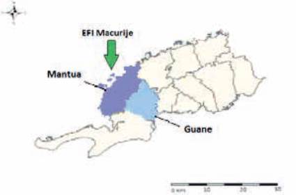
The "Macurije" Agroforestry Company is located in the westernmost region of Pinar del Rio province, covering parts of the territories of the municipalities of Guane and Mantua ^{(Valdés et al., 2021)}. It is bordered to the north by the coastal from the Baja inlet to the Garnacha inlet; to the east by the municipality of San Juan y Martinez, belonging to the Empresa Agroforestal Pinar del Rio (EAF); to the south by the municipality of Sandino Empresa Agroforestal Guanacahabibes (EAF); and to the southeast by the Gulf of Mexico.

The study was developed in natural stands of Pinus caribaea var. caribaea, subjected to clear-cutting, where the average diameter of the trees was 24.6 cm, the height was 15.3 m and the average volume of the trees was 0.31 m3, the total volume was 125 m³ ha-1. The average annual temperature of the site is 23.8°C, the relative humidity is 74 % and the average annual rainfall is 1,486.6 mm. The terrain has an undulating relief, with slopes between 12 and 28 %. The soil is classified as sandy clay loam.

The harvesting system used during the development of this study is long logs (Machado et al., 2014; Guera 2016). For the development of the application, we worked on Windows 7 Professional operating system, the development environment used was Microsoft Visual Studio 2008 and the database management system, Microsoft Access. In addition, version 3.5 of the ASP.Net framework for Web applications was used and C++ was chosen as the programming language, being the language designed by Microsoft for its .NET platform.

The COSTOFOR application has two modules of work, related to each other and operated sequentially.

Determination of the number of samples

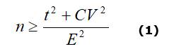
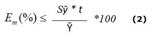
The initial (pilot) sample used in the study was 45 operating cycles for each of the wood extraction means. The minimum number of operating cycles required per extraction equipment to obtain a certain precision, prefixed by a maximum allowable sampling error of 10 % was determined from equation (1) according to ^{Guera et al. (2020)}. The sampling errors were determined by (Equation 1 and Equation 2).

Where:

n	- Minimum number of operating cycles required for each extraction machine or equipment
t	- student's t-value (gl=n - 1; 1 - á = 0.95)
CV	(%) - coefficient of variation
E	- Permissible error (10 %)
Sï	- standard deviation of the mean
2	- sample mean

Determination of the costs of the harvesting system

The cost of the harvesting system was calculated and the optimization criteria costs were implemented ^{(Santos et al., 2016)}, the selection of the most effective technological variant, the selection of the optimal size of the working group ^{(Guera et al., 2020)}, as well as the determination of the optimal density of roads and stockpiles ^{(Ferraço de Campos et al., 2017)}.

For this purpose, a high- performance technological evaluation of the equipment was carried out, which made it possible to calculate the operating cost, the utilization of the machines and its performance. By operating costs we mean property or fixed costs, (depreciation cost, interest cost, insurance cost and tax cost), operating costs (fuel cost, lubricant cost, repair and maintenance cost, cost of other materials) and workforce costs (direct salaries received by machine operators and helpers, adding to these the indirect costs of social charges, such as benefits, supervision and safety). Road and loading yard construction costs are also updated. In order to do so, different activities to be developed during the exploitation process were defined (planning, strip cleaning, embankment, formation, drainage, profiling and loading yards), the sub-activities (which in the application can be found as sub-operations) within each activity and the regulations, and the property, operation and labor costs are recalculated ^{(Candano et al., 2015)}.

Unit costs were also updated, dividing the cost of operating the machines by the performance of these in the different operations that include cutting or felling, delimbing, cutting, logging, extraction, loading, transport, and road and loading yard construction. To do this, it was necessary to calculate the productivity (Rh), using the (Equation 3).

Once the cost of the harvesting system was calculated, the optimal density of roads and stockpiles was determined (expression 6), in which the optimal criterion is the minimum of the sum of the cost of road construction and hauling cost. For this purpose, an interaction between the expression was used for calculating the unit cost of hauling and the unit cost of roads and loading yards. To calculate the cost per unit of production, the expression (4) was used for roads and loading yards, and expression (5) was used for hauling, as described by Candano et al. (2011) (Equation 4):

Where:

Cuc	- Unit cost of roads and freight yards ($/m3)
Cr	- Cost of road construction ($/km)
V	- Volume of wood used per unit area (m3/ha)
Cl	- Yard construction cost ($)
L	- Average yard spacing (m)
S	- Average spacing between roads (m)

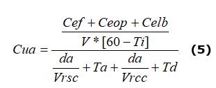
The following expression was used to calculate the cost of wood hauling (Equation 5):

Where:

Cua	- Unit cost of wood hauling ($/m3)
Cef	- Tractor fixed cost ($/h)
Ceop	- Tractor variable cost ($/h)
Celb	- Labor cost ($/h)
V	- Tractor trailed volume or payload (m3)
Ti	- Interruption time (min/h)
da	- Average drag distance (m)
Vrsc	- Unladen tractor speed (m/min)
Vrcc	- Tractor loaded speed (m/min)
Ta	- Timber lashing time (min.)
Td	- Time of untying (min)

As the hauling distance (hd), is a function of the average spacing between roads and between yards, and intervenes in the cost of road construction and also in the cost of hauling, the expression (6) was used, which serves as an interaction between both operations (Equation 6):

The average hauling distance in expression (5) contains the average road spacing (S) and the average yard spacing (L). Then the cost of roads and the hauling cost will be determined by these two variables (S and L). The variable k is the sinuosity coefficient, (k ≥ 1), the ratio of the actual hauling distance to the theoretical distance.

As there are many possible interactions, an algorithm was created to automate these calculations and to determine the optimal average spacing between roads and between loading yards, and at the same time a hauling distance that achieves a minimum cost for both operations.

The algorithm includes a programmed cycle. For the spacing between roads, it has a diapason from 100 to 1650 meters with a step of 50m, and for the cycle of the spacing between yards, values from 50 to 375 with a step of 25m were taken. Once the optimal criterion is calculated, the values obtained are substituted and the cost of hauling and the cost of road and yard construction are recalculated, which implies a decrease in the cost of the harvesting system.

Financial analysis of the utilization

First, the value of the initial investment was updated, since it is a parameter that is taken into account for the financial analysis and on its amount depends the result of the net present value (NPV) and the investment recovery period (IRP). In this case, the purchase price of the newly acquired equipment that will be implemented in the use of the selected area was updated, the repairs and also the technical and organizational market study, environmental license and working capital.

The Cost-Benefit (C/B) ratio directly compares benefits and costs. To calculate the C/B ratio, first find the sum of the discounted benefits, brought to the present, which in our case is the resulting value of the standing timber potential in a previously selected area, and divide it by the sum of the discounted costs, which is the amount of the cost of the harvesting system, according to the variant used ^{(Ucañan 2020)} .

For a conclusion about the feasibility of a project, under this approach, the comparison of the C/B ratio found compared to 1 should be taken into account, thus we have the following:

• C/B > 1 indicates that the benefits exceed the costs, therefore the project should be considered.

• C/B =1 Here there are no gains, since the benefits are equal to the costs.

• C/B < 1, shows that the costs are greater than the benefits, it should not be considered.

To perform the analysis of the economic indicators, the evaluated area and unit cost variant are requested. From the calculated analysis, the system gives the possibility to break down the parameters or elements in the years of use, and in turn to calculate the indicators: NPV, ERP and the C/B Ratio.

The Net Present Value (NPV) of an investment or investment project is a measure of the absolute net profitability provided by the project. At the initial moment of the project, the increase in value provided to the owners in absolute terms is measured, once the initial investment that had to be made to carry it out has been discounted. The expression for the calculation of NPV according to Granel (2021) is as follows (Equation 7):

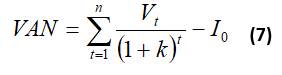
Where:

I 0	- value of the initial disbursement of the investment
V t	- represents the cash flows (in our case we consider the net liquidity) in each period t
K	- discount rate
N	- number of periods considered

Another parameter to be quantified for this analysis is the percentage of opportunity cost, which is defined as the cost of the alternative that is renounced when a certain decision is made, including the benefits that could have been obtained if the alternative option had been chosen. The discount rate variable is also used.

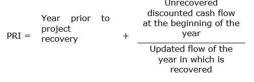
The Investment Recovery Period (IRP) is an indicator that measures how long it will take to recover the total investment at present value. It can reveal precisely, in years, months and days, the date on which the initial investment will be covered. Its expression is (Equation 8):

A Web application (COSTOFOR) was successfully programmed, which makes it possible to: provide editing, visualization and information exchange tools; estimate the value of standing timber potential, based on information recorded in the field inventory and information on the current price of timber on the market; calculate and optimize the costs of forest harvesting technologies or exploitation costs (ownership, operation and labor), as well as the costs of road and loading yard construction for each of the activities to be carried out (survey, clearing, embankment, drainage, surface and loading yards), unit costs per operation (felling, and apply economic-financial indicators (cost-benefit ratio, net present value and investment recovery period) that allow us to define the economic viability of the project analyzed and simulated, the profitability of the investment, and make decisions based on the results obtained.

Based on a previous analysis of the standing timber potential in a given area, the values of the variables are updated to calculate the fixed costs (depreciation cost, interest cost, insurance cost and tax cost) and the total fixed cost is calculated. The values of the variables are updated to calculate the operating costs (fuel cost, lubricant cost, repair and maintenance cost, cost of other materials), according to the groups of equipment: cutting tools, truck, tractor and animal, and the total operating cost is calculated. The values of the variables are also updated to calculate labor costs (direct salaries received by machine operators and assistants, adding to these the indirect costs of social charges, such as benefits, supervision and safety) ^{(Guera et al., 2020)}.

RESULTS AND DISCUSSION

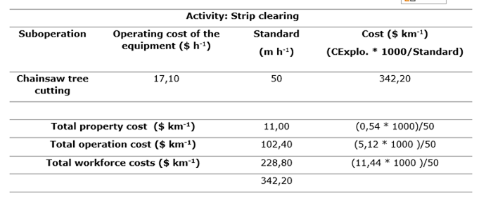
Road and loading yard construction costs were obtained. The activities to be developed during the harvesting process were also defined (planning, strip clearing, embankment, formation, drainage, profiling and loading yards), the sub-operations (tree cutting with chainsaws, skidding, cover vegetation removal, among others) within each activity and the regulations, and the costs of ownership, operation and labor were recalculated. The recalculated cost is obtained by dividing the operating cost of the equipment by the regulation, but the operating cost is expressed in $/h, while the recalculated cost is expressed in $ km-1, which is why for an operating cost of $17.10 h-1 with a regulation of 50 m h-1, $342.20 km-1 are obtained (Table 1). These results are similar to the studies of ^{Candano et al. (2015}) and Guera (2016).

Table 1 Results obtained from the calculation of forest road construction costs 

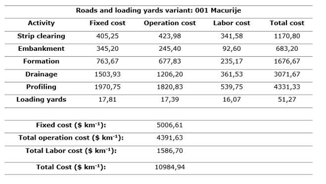
A summary table of road and loading yard construction costs by activity is presented in Table 2, once all the activities and sub-activities to be developed in this variant have been updated.

Table 2.  -Summary of road and freight yard construction costs 

The other cost to be calculated is the unit cost. When calculating the unit cost for chainsaw logging, an operating cost of $17.10 $ h^-1 was considered, of which $ 0.54 corresponds to the cost of ownership, $ 5.12 to the cost of operation and $ 11.44 to the cost of labor. The average volume of trees is of 0.70 m³, interruption time of 8 min/h and cutting time of 5 min tree^-1(Equation 9).

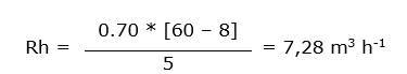
• CU property = 0,54 / 7,28 = 0,08

• CU operation = 5,12/7,28 = 0,70

• CU labor = 11,44 / 7.28 = 1,57

• CU Total = 2,35

Table 3.  - Summary table of unit costs 

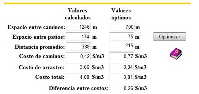
A summary table by operation is shown in Table 3, for the specified variant. Once the cost of the harvesting system was calculated, the optimum criterion was applied using the expression that serves as an interaction between the cost of road construction and the cost of haulage. From the following example, we calculate values of spacing between roads S = 1 246 m and spacing between yards L equal to 174 m, and we establish a comparison between calculated values and optimal values. For the variable k (sinuosity coefficient) a value of 1.2 was taken. As shown in Figure 2, the cost of roads increased by 0.34 $ m^-3, the cost of extraction (hauling) decreased by 0.62 $ m^-3, which finally influences a slight decrease of 0.27 $ m^-3 of the total cost, which represents that for every 1 000 m³ harvested, $ 270 is saved or wasted.

Fig. 2.  - User interface. Comparison between calculated and optimal values 

Finally, if the value of the evaluated timber potential and the value of the harvesting cost are already available, the financial analysis can be made on the basis of these results.

An example of what the application should show in terms of calculating the cost/benefit ratio is shown in Table 4.

Table 4.  - Example of the calculation of the cost-benefit ratio 

Concepts
Income	2 748 500.00
Total expenditures	2 482 194.00
Operating expenses	2 256 540.00
10% Administrative Expenses	225 654.00
Other expenses	0.00
Incomes befores taxes	266 556.00
35% Taxes:	93 294.60
Net Income	173 261.40
Cost/Profit:	1.07

Since the Cost/Benefit (C/B) ratio is > 1, the benefits exceed the costs and, therefore, the project should be considered.

Other indicators analyzed are the Net Present Value (NPV) and the Payback Period (PRI). Starting in the same way as the previous example, the application performs the following analysis.

It is assumed that we are planning for 10 years of utilization. For Year 0, we start from the value of the initial investment Io = $ 692,700.00, whose opportunity cost is $69,270.00 (10%). The total expenses for that year will be -$ 761,970.00, taking into account that in that year there is no income, and that constitutes the Net Liquidation for that year, and the cash flows (Net Liquidity) from Year 1 will be: V1, V2, V3, V4, V5, V6, V7, V8, V9 and V10 = $17 326.14 (274 875.00-(248 219.40 + 9 329.46)). The income, expenses and tax are spread equally over the 10 years.

The factor (1+k)t for Year 1 will be (1+0.15)1 = 1.15, so the first addendum will then be $17 326.14 /1.15 = $15 066.21. The accumulated liquidation for that year will be $17 326.14 - 761 970.00 = -$ 744 643.86. Each year the factor (1+k)^t is increased and the sum takes on a new value. The summation in the Net Present Value (NPV) formula increases and the amount reached at Year 10 and deducting the value of the initial investment, gives us the NPV value. An NPV > 0 means that the project can be accepted as economically viable.

In this case, as the results for Year 1 show, it will be impossible to obtain a positive NPV for 10 years of use, therefore, the project is not economically viable. The example is proposed with every intention.

The same should be true for the Payback Period (PRI), considering that the annual net liquidation is much lower than the initial investment made.

Let us assume the same Total Expense for Year 0 of -$761,970.00 and a Net Liquidation each year of $324,746.38.

To calculate the year prior to project recovery, the following analysis is performed:

• Year 1: -761 970.00 + (324 746.38 / (1+0.15)) = -761 970.00 + 282 388.16 = -479 581.84 (no recovery).

• Year 2: -479 581.84 + (324 746.38 / (1+0.15)2) = -479 581.84 + 245 554.92 = -234 026.92 (no recovery).

• Year 3: -234 026.92 + (324 746.38 / (1+0.15)3) = -234 026.92 + 213 522.51 = -20 504.41 (no recovery).

• Year 4: -20 504.41 + (324 746.38 / (1+0.15)4) = -20 504.41 + 185 675.46 = 165 171.05 (recoverable).

Therefore:

• Year prior to project recovery = 3.

• Unrecovered discounted cash flow at the beginning of the year = 20 504,41.

• Recovered discounted cash flow in the year of recovery = 185,675.46.

• The PRI formula is applied and PRI = 3.11.

From there, take the decimal part, i.e. 0.11, and multiply it by 12 (months) and you get 1.32, which means 1 month and a little more. Take the decimal part, i.e. 0.32 and multiply it by 30 (days) and you get 9.6, which means 9 days. Therefore, it is concluded that the PRI is 3 years, 1 month and 9 days.

CONCLUSIONS

This tool allows business management and enables the simulation of the utilization process before planning, allowing the selection of the best alternative according to the current conditions.

From the economic point of view, it allows minimizing the cost of the utilization system, guaranteeing a minimum cost and an increase in the profitability of the system, and the simulation of the utilization process by reducing the amount of resources to be used through the implementation of optimization criteria.

REFERENCIAS BIBLIOGRÁFICAS

CÁNDANO, F., PEÑALVER, A., RAMOS, M. P., DRESCHER, P. 2015. Densidad óptima de caminos y acopiaderos en el manejo de bosques naturales en Mato Grosso, Brasil. Espamciencia, v. 6, n. 1, pp. 97-103. http://revistasespam.espam.edu.ec/index.php/Revista_ESPAMCIENCIA/article/view/98

CANDANO, F., OLIVEIRA, D. C., ARRUDA, C., GARCIA, M. L., MELO, R. R. 2018. Operational Performance of the Selective Cutting of Trees with Chainsaw. Floresta e Ambiente V. 25, N. 3: e20160239 https://doi.org/10.1590/2179-8087.023916

FERRAÇAO DE CAMPOS, R., FIELDLER, N. C., PENETRA, J. L., DOS SANTOS, A. R., ASSIS, F., BOLDRINI, S., 2017. Densidade de estradas florestais em propriedades rurais. ACSA, Patos-PB, v.13, n.1, pp.59-66, janeiro-março. http://revistas.ufcg.edu.br/acsa/index.php/ACSA/index

GUERA, O. G. M., SILVA, A., FERREIRA, R. L., LAZO, D., MEDEL, H., 2019. Simulações de desbastes em plantios de Pinus caribaea Morelet var. caribaea Barrett & Golfari BIOFIX Scientific Journal v. 4, n. 2, pp. 146-152. DOI: dx.doi.org/10.5380/biofix.v4i2.65070

GUERA, O. G. M., SILVA, A., FERREIRA, R. C., ALVAREZ, D., BARRERO, H., DIAZ, A. 2020. Enfoque multivariado en experimentos de extracción de madera en plantaciones forestales. Madera y Bosques, v.26, n. 2, e2621934. Doi: 10.21829/myb.2020.2621934

PEREIRA, M. M., et al. 2017. Densidad óptima de caminos forestales con la extracción 1 de madera de Eucalyptus para clambunk skidder. 7^O Congreso Forestal Español. Gestión del monte: servicios ambientales y bioeconomía. SECF. . https://www.researchgate.net/publication/328096969_DENSIDAD_OPTIMA_DE_CAMINOS_FORESTALES_CON_LA_EXTRACCION_DE_MADERA_DE_Eucalyptus_PARA_CLAMBUNK_SKIDDER

SANTOS, L. N., et al 2016. Avaliação de custos da operação de extração da madeira com forwarder. CERNE, v. 22, n. 1, pp. 27-34. https://doi.org/10.1590/01047760201622012076

UCAÑAN, R. 2020. Relación Beneficio Costo (B/C): ejemplo en Excel. Recuperado de https://www.gestiopolis.com/calculo-de-la-relacion-beneficio-coste/

VALDES, R. H., ÁLVAREZ, D., y FERNÁNDEZ, R. R., 2021. Análisis de la calidad superficial de diferentes maderas. Revista Avances, v. 23, n. 2, 20-21. http://www.ciget.pinar.cu/ojs/index.php/publicaciones/article/view/612

VILLALOBOS, V., y MEZA, A., 2016. Evaluación de la etapa de arrastre en un aprovechamiento de plantaciones forestales de Acacia (Acacia mangium). San Carlos, Alajuela, Costa Rica. Revista Forestal Mesoamericana Kurú, v. 13, n. 33, pp. 3-10. http://DOI: 10.18845/rfmk.v13i33.2572

Received: May 17, 2022; Accepted: July 20, 2022

^*Autor para la correspondencia: [e-mail]

Los autores declaran no tener conflictos de intereses.

Los autores han participado en la redacción del trabajo y análisis de los documentos.