<?xml version="1.0" encoding="ISO-8859-1"?><article xmlns:mml="http://www.w3.org/1998/Math/MathML" xmlns:xlink="http://www.w3.org/1999/xlink" xmlns:xsi="http://www.w3.org/2001/XMLSchema-instance">
<front>
<journal-meta>
<journal-id>1815-5928</journal-id>
<journal-title><![CDATA[Ingeniería Electrónica, Automática y Comunicaciones]]></journal-title>
<abbrev-journal-title><![CDATA[EAC]]></abbrev-journal-title>
<issn>1815-5928</issn>
<publisher>
<publisher-name><![CDATA[Universidad Tecnológica de La Habana José Antonio Echeverría, Cujae]]></publisher-name>
</publisher>
</journal-meta>
<article-meta>
<article-id>S1815-59282017000100008</article-id>
<title-group>
<article-title xml:lang="en"><![CDATA[Optimal Predefined-Time Stabilization for a Class of Linear Systems]]></article-title>
<article-title xml:lang="es"><![CDATA[Estabilización de tiempo predefinido óptima para una clase de sistemas lineales]]></article-title>
</title-group>
<contrib-group>
<contrib contrib-type="author">
<name>
<surname><![CDATA[Jiménez-Rodríguez]]></surname>
<given-names><![CDATA[Esteban]]></given-names>
</name>
<xref ref-type="aff" rid="A01"/>
</contrib>
<contrib contrib-type="author">
<name>
<surname><![CDATA[Sánchez-Torres]]></surname>
<given-names><![CDATA[Juan Diego]]></given-names>
</name>
<xref ref-type="aff" rid="A02"/>
</contrib>
<contrib contrib-type="author">
<name>
<surname><![CDATA[Loukianov]]></surname>
<given-names><![CDATA[Alexander G.]]></given-names>
</name>
<xref ref-type="aff" rid="A01"/>
</contrib>
</contrib-group>
<aff id="A01">
<institution><![CDATA[,Advanced Studies and Research Center of the National Polytechnic Institute (CINVESTAV)  ]]></institution>
<addr-line><![CDATA[Guadalajara ]]></addr-line>
<country>México</country>
</aff>
<aff id="A02">
<institution><![CDATA[,ITESO University Department of Mathematics and Physics ]]></institution>
<addr-line><![CDATA[Guadalajara ]]></addr-line>
<country>México</country>
</aff>
<pub-date pub-type="pub">
<day>00</day>
<month>04</month>
<year>2017</year>
</pub-date>
<pub-date pub-type="epub">
<day>00</day>
<month>04</month>
<year>2017</year>
</pub-date>
<volume>38</volume>
<numero>1</numero>
<fpage>90</fpage>
<lpage>101</lpage>
<copyright-statement/>
<copyright-year/>
<self-uri xlink:href="http://scielo.sld.cu/scielo.php?script=sci_arttext&amp;pid=S1815-59282017000100008&amp;lng=en&amp;nrm=iso"></self-uri><self-uri xlink:href="http://scielo.sld.cu/scielo.php?script=sci_abstract&amp;pid=S1815-59282017000100008&amp;lng=en&amp;nrm=iso"></self-uri><self-uri xlink:href="http://scielo.sld.cu/scielo.php?script=sci_pdf&amp;pid=S1815-59282017000100008&amp;lng=en&amp;nrm=iso"></self-uri><abstract abstract-type="short" xml:lang="en"><p><![CDATA[This paper addresses the problem of optimal predefined-time stability. Predefined-time stable systems are a class of fixed-time stable dynamical systems for which a bound of the settling-time function can be defined a priori as an explicit parameter of the system. Sufficient conditions for a controller to solve the optimal predefined-time stabilization problem for a given nonlinear system are provided. Furthermore, for nonlinear affine systems and a specific performance index, a family of inverse optimal predefined-time stabilizing controllers is derived. This class of controllers is applied to the inverse predefined-time optimization of the sliding manifold reaching phase in linear systems, jointly with the idea of integral sliding mode control to ensure robustness. Finally, as a study case, the developed methods are applied to an uncertain satellite system, and numerical simulations are carried out to show their behavior.]]></p></abstract>
<abstract abstract-type="short" xml:lang="es"><p><![CDATA[Este trabajo trata el problema de estabilidad óptima en tiempo predefinido. Los sistemas estables en tiempo predefinido son una clase de sistemas que presentan la propiedad de estabilidad en tiempo fijo y, además, una cota de la función de tiempo de convergencia puede ser definida a priori como un parámetro explícito del sistema. En el trabajo se proporcionan condiciones suficientes para que el problema de estabilización optima en tiempo predefinido sea soluble dado un sistema no lineal. Además, para sistemas no lineales afines al control y un índice de desempeño específico, se deriva una familia de controladores estabilizantes en tiempo predefinido. Esta clase de controladores se aplica a la optimización inversa en tiempo predefinido de la fase de alcance de variedades deslizantes en sistemas lineales, junto con la idea de modos deslizantes integrales para brindar robustez. Finalmente, como caso de estudio, los métodos desarrollados se aplican a un sistema de satélite con incertidumbre, y se llevan a cabo simulaciones numéricas para validar su comportamiento.]]></p></abstract>
<kwd-group>
<kwd lng="en"><![CDATA[Hamilton-Jacobi-Bellman Equation]]></kwd>
<kwd lng="en"><![CDATA[Lyapunov Functions]]></kwd>
<kwd lng="en"><![CDATA[Optimal Control]]></kwd>
<kwd lng="en"><![CDATA[Predefined-Time Stability]]></kwd>
<kwd lng="es"><![CDATA[Ecuación de Hamilton-Jacobi-Bellman]]></kwd>
<kwd lng="es"><![CDATA[Funciones de Lyapunov]]></kwd>
<kwd lng="es"><![CDATA[Control Óptimo]]></kwd>
<kwd lng="es"><![CDATA[Estabilidad de tiempo predefinido]]></kwd>
</kwd-group>
</article-meta>
</front><body><![CDATA[  	    <p align="right"><font face="Verdana" size="2"> <b>ORIGINAL ARTICLE</b></font></p>     <p align="justify">&nbsp;</p>     <p align="justify">&nbsp; </p> 	    <p align="justify"><font face="verdana" size="4"><strong>Optimal Predefined&#45;Time Stabilization for a Class of Linear Systems</strong></font></p> 	    <p align="justify">&nbsp;</p> 	    <p align="justify"><font face="verdana" size="3"><b>Estabilizaci&oacute;n de tiempo predefinido &oacute;ptima para una clase de sistemas lineales</b></font></p>  	    <p align="justify">&nbsp;</p> 	    <p align="justify">&nbsp;</p> 	    <p align="justify"><font face="verdana" size="2"><strong>Esteban Jim&eacute;nez&#45;Rodr&iacute;guez <sup>I</sup>, Juan Diego S&aacute;nchez&#45;Torres <sup>II</sup>, Alexander G. Loukianov <sup>I</sup></strong><sup></sup></font></p>  	     ]]></body>
<body><![CDATA[<p align="justify"><font face="verdana" size="2"><sup>I</sup> Advanced Studies    and Research Center of the National Polytechnic Institute (CINVESTAV). Guadalajara,    M&eacute;xico.    <br>   <sup>II</sup> Department of Mathematics and Physics of ITESO University. Guadalajara,    M&eacute;xico.</font></p>      <p align="justify">&nbsp;</p>     <p align="justify">&nbsp;</p> <hr align="JUSTIFY" size="1" noshade>  	    <p align="justify"><font face="verdana" size="2"><strong>ABSTRACT</strong></font></p>  	    <p align="justify"><font face="verdana" size="2">This paper addresses the problem of optimal predefined&#45;time stability. Predefined&#45;time stable systems are a class of fixed&#45;time stable dynamical systems for which a bound of the settling&#45;time function can be defined a priori as an explicit parameter of the system. Sufficient conditions for a controller to solve the optimal predefined&#45;time stabilization problem for a given nonlinear system are provided. Furthermore, for nonlinear affine systems and a specific performance index, a family of inverse optimal predefined&#45;time stabilizing controllers is derived. This class of controllers is applied to the inverse predefined&#45;time optimization of the sliding manifold reaching phase in linear systems, jointly with the idea of integral sliding mode control to ensure robustness. Finally, as a study case, the developed methods are applied to an uncertain satellite system, and numerical simulations are carried out to show their behavior.</font></p>  	     <p align="justify"><font face="verdana" size="2"><b>Key words:</b> Hamilton&#45;Jacobi&#45;Bellman    Equation, Lyapunov Functions, Optimal Control, Predefined&#45;Time Stability.</font></p>  	<hr align="JUSTIFY" size="1" noshade>     <p align="justify"><font face="verdana" size="2"><b>RESUMEN</b></font></p>  	     <p align="justify"><font face="verdana" size="2">Este trabajo trata el problema    de estabilidad &oacute;ptima en tiempo predefinido. Los sistemas estables en    tiempo predefinido son una clase de sistemas&nbsp; que presentan la propiedad&nbsp;    de estabilidad en tiempo fijo y, adem&aacute;s, una cota de la funci&oacute;n    de tiempo de convergencia puede ser definida a priori como un par&aacute;metro    expl&iacute;cito del sistema. En el trabajo se proporcionan condiciones suficientes    para que el problema de estabilizaci&oacute;n optima en tiempo predefinido sea    soluble dado un sistema no lineal. Adem&aacute;s, para sistemas no lineales    afines al control y un &iacute;ndice de desempe&ntilde;o espec&iacute;fico,    se deriva una familia de controladores estabilizantes en tiempo predefinido.    Esta clase de controladores se aplica a la optimizaci&oacute;n inversa en tiempo    predefinido de la fase de alcance de variedades deslizantes en sistemas lineales,    junto con la idea de modos deslizantes integrales para brindar robustez. Finalmente,    como caso de estudio, los m&eacute;todos desarrollados se aplican a un sistema    de sat&eacute;lite con incertidumbre, y se llevan a cabo simulaciones num&eacute;ricas    para validar su comportamiento.</font></p>  	    <p align="justify"><font face="verdana" size="2"><b>Palabras Claves:</b> Ecuaci&oacute;n de Hamilton&#45;Jacobi&#45;Bellman, Funciones de Lyapunov, Control &Oacute;ptimo, Estabilidad de tiempo predefinido</font></p>  <hr align="JUSTIFY" size="1" noshade>     ]]></body>
<body><![CDATA[<p align="justify">&nbsp;</p>     <p align="justify">&nbsp;</p>     <p align="justify"><font face="verdana" size="3"><b>1.&#45;</b> <b>INTRODUCTION</b></font></p>     <p align="justify">&nbsp;</p>  	    <p align="justify"><font face="verdana" size="2">Finite&#45;time stable dynamical systems provide solutions to applications which require hard time response constraints. Important works involving the definition and application of finite&#45;time stability have been carried out in &#91;1&#45;5&#93; Nevertheless, this finite stabilization time is often an unbounded function of the initial conditions of the system. Making this function bounded to ensure the settling time is less than a certain quantity for any initial condition may be convenient, for instance, for optimization and state estimation tasks. With this purpose, a stronger form of stability, in which the convergence time presents a class of uniformity with respect to the initial conditions, called <i>fixed&#45;time stability</i> was introduced &#91;6&#45;9&#93;. When fixed&#45;time stable dynamical systems are applied to control or observation, it may be difficult to find a direct relationship between the gains of the system and the upper bound of the convergence time; thus, tuning the system in order to achieve a desired maximum stabilization time is not a trivial task.</font></p>  	    <p align="justify"><font face="verdana" size="2">In this sense, another class of dynamical systems which exhibit the property of <i>predefined&#45;time stability</i>, have been studied &#91;10,11&#93;. For these systems, an upper bound of the convergence time appears explicitly in their dynamical equations; in particular, it equals the reciprocal of the system gain. Moreover, for unperturbed systems, this bound is not a conservative estimation but truly the minimum value that is greater than all the possible exact settling times.</font></p>  	    <p align="justify"><font face="verdana" size="2">On the other hand, the infinite&#45;horizon, nonlinear non&#45;quadratic optimal asymptotic stabilization problem was addressed in &#91;12&#93;. The main idea of the results are based on the condition that a Lyapunov function for the nonlinear system is at the same time the solution of the steady&#45;state Hamilton&#45;Jacobi&#45;Bellman equation, guaranteeing both asymptotic stability and optimality. Nevertheless, returning to the first paragraph idea, the finite&#45;time stability is a desired property in some applications, but optimal finite&#45;time controllers obtained using the maximum principle do not generally yield feedback controllers. In this sense, the optimal finite&#45;time stabilization is studied in &#91;13&#93;, as an extension of &#91;12&#93;. Since the results are based on the framework developed in &#91;12&#93;, the controllers obtained are feedback controllers.</font></p>  	    <p align="justify"><font face="verdana" size="2">Consequently, as an extension of the ideas presented in &#91;11&#45;14&#93;, this paper addresses the problem of <i>optimal predefined&#45;time stabilization</i>, namely the problem of finding a state&#45;feedback control that minimizes certain performance measure, guaranteeing at the same time predefined&#45;time stability of the closed&#45;loop system. In particular, sufficient conditions for a controller to solve the optimal predefined&#45;time stabilization problem for a given system are provided. These conditions involve a Lyapunov function that satisfy both a certain differential inequality for guaranteeing predefined&#45;time stability and the steady&#45;state Hamilton&#45;Jacobi&#45;Bellman equation for ensuring optimality. Furthermore, this result is applied to the predefined&#45;time optimization of the sliding manifold reaching phase in linear systems, jointly with the integral sliding mode control idea to provide robustness. Finally, as a study case, the predefined&#45;time optimization of the sliding manifold reaching phase in an uncertain satellite system is performed using the developed methods, and numerical simulations are carried out to show their behavior.</font></p>  	    <p align="justify">&nbsp;</p>  	    <p align="justify"><font face="verdana" size="3"><b>2.&#45; MATHEMATICAL PRELIMINARES: PREDEFINED&#45;TIME STABILITY</b></font></p> 	    ]]></body>
<body><![CDATA[<p align="justify">&nbsp;</p> 	    <p align="justify"><font face="verdana" size="2">Consider the system</font></p>  	    <p align="justify"><a name="ec1"/><img src="/img/revistas/eac/v38n1/e0108117.gif">  	    <p align="justify"><font face="verdana" size="2">where x &#8712; &#8476;<sup>n</sup> is the system state, &#961; &#8712; &#8476;<sup>b</sup> stands for the system parameters and f:&#8476;<sup>n</sup>&#8594;&#8476;<sup>n</sup> is a function such that f(0)=0, i.e. the origin x=0 is an equilibrium point of <a href="#ec1">(1)</a>.</font></p>  	    <p align="justify"><font face="verdana" size="2"><i>Definition 1.1</i>. &#91;8&#93; The origin of <a href="#ec1">(1)</a> is globally finite&#45;time stable if it is globally asymptotically stable and any solution x(t,x<sub>0</sub>) of <a href="#ec1">(1)</a> reaches the equilibrium point at some finite time moment, i.e., &#8704; t &#8805; T(x<sub>0</sub>):x(t,x<sub>0</sub>)=0, where T: &#8476;<sup>n</sup>&#8594;&#8476;<sub>+</sub> &#8746; {0}.</font></p>  	    <p align="justify"><font face="verdana" size="2"><i>Remark 1.1</i>. The settling&#45;time function T(x<sub>0</sub>) for systems with a finite&#45;time stable equilibrium point is usually an unbounded function of the system initial condition.</font></p>  	    <p align="justify"><font face="verdana" size="2"><i>Definition 1.2</i>. &#91;8&#93; The origin of the system (1) is fixed&#45;time stable if it is globally finite&#45;time stable and the settling&#45;time function is bounded, i.e. &#8707; T<sub>max</sub> &gt; 0:&#8704; x<sub>0</sub>&#8712; &#8476;<sup>n</sup>: T(x<sub>0</sub>)&#8804; T<sub>max.</sub></font></p>  	    <p align="justify"><font face="verdana" size="2"><i>Remark 1.3.</i> Note that there are several choices for T<sub>max</sub>. For instance, if the settling&#45;time function is bounded by T<sub>m</sub>, it is also bounded by &#955;T<sub>m</sub> for all &#955;&#8805;1. This motivates the following definition.</font></p>  	    <p align="justify"><font face="verdana" size="2"><i>Definition 1.3</i>. &#91;11&#93; Assume that the origin of the system <a href="#ec1">(1)</a> is fixed&#45;time stable. Let &#932; be the set of all the bounds of the settling&#45;time function for the system <a href="#ec1">(1)</a>, i.e.,</font></p>  	    <p align="justify"><a name="ec2"/>     	  <img src="/img/revistas/eac/v38n1/e0208117.gif"> 	    ]]></body>
<body><![CDATA[<p align="justify"><font face="verdana" size="2">Then, the minimum bound of the settling&#45;time function T<sub>f</sub>, is defined as</font></p>  	    <p align="justify"><a name="ec3"/><img src="/img/revistas/eac/v38n1/e0308117.gif">  	    <p align="justify"><font face="verdana" size="2"><i>Remark 1.2</i>. The time T<sub>f</sub> in the above definition can be considered as the true fixed&#45;time in which the system (1) is stabilized.</font></p>  	    <p align="justify"><font face="verdana" size="2"><i>Definition 1.4.</i> &#91;11&#93; For the case of fixed&#45;time stability when the system <a href="#ec1">(1)</a> parameters &#961; can be expressed in terms of&nbsp; T<sub>max</sub> or T<sub>f</sub> (a bound or the least upper bound of the settling&#45;time function), it is said that the origin of the system <a href="#ec1">(1)</a> is <i>predefined&#45;time stable</i>.</font></p>  	    <p align="justify"><font face="verdana" size="2">With the above definition, the following lemma provides a Lyapunov&#45;like condition for predefined&#45;time stability of the origin:</font></p>  	    <p align="justify"><font face="verdana" size="2"><i>Lemma 1.1</i>. &#91;10&#93; Assume there exist a continuous radially unbounded function V: &#8476;<sup>n</sup>&#8594;&#8476;<sub>+</sub> &#8746; {0}, and real numbers T<sub>c</sub> &gt;0 and 0&lt;p&#8804;1, such that the system <a href="#ec1">(1)</a> parameters &#961; can be expressed as a function of T<sub>c</sub> &gt;0, and</font></p>  	    <p align="justify"><a name="ec4"/><img src="/img/revistas/eac/v38n1/e0408117.gif"> 	    <p align="justify"><a name="ec5"/><img src="/img/revistas/eac/v38n1/e0508117.gif">  	    <p align="justify"><font face="verdana" size="2">and the time derivative of <i>V</i> along the trajectories of the system <a href="#ec1">(1)</a> satisfies the differential inequality</font></p>  	    <p align="justify"><a name="ec6"/><img src="/img/revistas/eac/v38n1/e0608117.gif">  	    ]]></body>
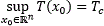
<body><![CDATA[<p align="justify"><font face="verdana" size="2">Then, the origin of the system <a href="#ec1">(1)</a> is predefined&#45;time stable with T(x<sub>0</sub>) &#8804; T<sub>c</sub>.</font></p>  	    <p align="justify"><font face="verdana" size="2"><i>Remark 1.3.</i> Lemma 1.1 characterizes fixed&#45;time stability in a very practical way since the condition <a href="#ec6">(6)</a> directly involves a bound on the convergence time. However, this condition is not sufficient for T<sub>c</sub> to be the least upper bound of the settling&#45;time function T(x<sub>0</sub>). A sufficient condition is provided in the following corollary of Lemma 1.1.</font></p>  	    <p align="justify"><font face="verdana" size="2"><i>Corollary 1.1.</i> Under the same conditions of Lemma 1.1, if the time derivative of <i>V</i> along the trajectories of the system <a href="#ec1">(1)</a> satisfies differential equation</font></p>  	    <p align="justify"><a name="ec7"/><img src="/img/revistas/eac/v38n1/e0708117.gif">  	    <p align="justify"><font face="verdana" size="2">then, the origin of the system <a href="#ec1">(1)</a> is predefined &#45;time stable with <img src="/img/revistas/eac/v38n1/i0108117.gif">.</font></p>  	    <p align="justify"><font face="verdana" size="2"><i>Remark 1.4.</i> Note that the equality condition <a href="#ec7">(7)</a> is more restrictive than the inequality <a href="#ec6">(6)</a>, in the sense that to obtain the equality in <a href="#ec7">(7)</a> no uncertainty in the system model is allowed.</font></p>  	    <p align="justify"><font face="verdana" size="2"><i>Definition 1.5</i>. &#91;11&#93; For x &#8712; &#8476;<sup>n</sup>, 0&lt;p&#8804;1 and T<sub>c</sub> &gt;0, the predefined&#45;time stabilizing function is defined as</font></p>  	    <p align="justify"><a name="ec8"/><img src="/img/revistas/eac/v38n1/e0808117.gif">  	    <p align="justify"><font face="verdana" size="2"><i>Remark 1.5</i>. The function &#934;<sub>p</sub>(x; T<sub>c</sub>) is continuous and non&#45;Lipschitz for 0&lt;p&lt;1, and discontinuous for p=1.</font></p>  	    <p align="justify"><font face="verdana" size="2">The following two lemmas give meaning to the name "<i>predefined&#45;time stabilizing function</i>".</font></p>  	    ]]></body>
<body><![CDATA[<p align="justify"><font face="verdana" size="2"><i>Lemma 1.2</i>. &#91;11&#93; For every initial condition x<sub>0</sub>, the origin of the system</font></p>  	    <p align="justify"><a name="ec9"/><img src="/img/revistas/eac/v38n1/e0908117.gif">  	    <p align="justify"><font face="verdana" size="2">with T<sub>c</sub> &gt;0, and 0&lt;p&#8804;1 is predefined&#45;time stable with <img src="/img/revistas/eac/v38n1/i0108117.gif">.</font></p>  	    <p align="justify"><font face="verdana" size="2">The previous results have been applied to design a robust predefined&#45;time controller for the perturbed system</font></p>  	    <p align="justify"><a name="ec10"/><img src="/img/revistas/eac/v38n1/e1008117.gif">  	    <p align="justify"><font face="verdana" size="2">with x, u &#8712; &#8476;<sup>n</sup> and &#916;: &#8476;<sub>+</sub> &times; &#8476;<sup>n</sup>&#8594;&#8476;<sup>n</sup>.&nbsp; The objective is to drive the system <a href="#ec10">(10)</a> state to the point x=0 in a predefined time, in spite of the unknown perturbation &#916;(t, x).</font></p>  	    <p align="justify"><font face="verdana" size="2"><i>Lemma 1.3</i>. &#91;11&#93; Let the function &#916;(t ,x) be considered as an unknown non&#45;vanishing perturbation bounded by |&#916;(t, x)|&#8804;&#948;, with 0&lt;&#948;&lt;&#8734;. Then, selecting the control input as</font></p>  	    <p align="justify"><a name="ec11"/><img src="/img/revistas/eac/v38n1/e1108117.gif">  	    <p align="justify"><font face="verdana" size="2">with T<sub>c</sub> &gt;0, 0&lt;p&lt;1 and k&#8805;&#948;, ensures&nbsp; the&nbsp; closed&#45;loop system <a href="#ec10">(10)</a>&#45;<a href="#ec11">(11)</a> origin is predefined&#45;time stable with T(x<sub>0</sub>) &#8804; T<sub>c</sub>.</font></p>  	    <p align="justify"><font face="verdana" size="2"><b>2.1.&#45; M</b><b>ATHEMATICAL PRELIMINARES: OPTIMAL CONTROL THEORY</b></font></p>  	    ]]></body>
<body><![CDATA[<p align="justify"><font face="verdana" size="2">Consider the controlled nonlinear system</font></p>  	    <p align="justify"><a name="ec12"/><img src="/img/revistas/eac/v38n1/e1208117.gif">  	    <p align="justify"><font face="verdana" size="2">where x &#8712; &#8476;<sup>n</sup> is the system state, u &#8712; &#8476;<sup>m</sup> is the system control input, which is restricted to belong to a certain set U &#8834; &#8476;<sup>m</sup> of the admissible controls, and f:&#8476;<sup>n</sup> &times; &#8476;<sup>m</sup> &#8594; &#8476;<sup>n</sup> is a nonlinear function with f(0,0)=0.</font></p>  	    <p align="justify"><font face="verdana" size="2">The control objective is to design a control law for the system <a href="#ec12">(12)</a> such that the following performance measure J(x<sub>0</sub>,u(&#8901;))=&#8747;<sub>0</sub><sup>tf</sup> L(x(t), u(t))dt is minimized. Here, L: &#8476;<sup>n</sup> &times; &#8476;<sup>m</sup> &#8594; &#8476; is a continuous function, assumed to be convex in u.</font></p>  	    <p align="justify"><font face="verdana" size="2">Define the minimum cost function J<sup>*</sup>(x(t), t) as</font></p>  	    <p align="justify"><a name="ec13"/><img src="/img/revistas/eac/v38n1/e1308117.gif">  	    <p align="justify"><font face="verdana" size="2">Then, defining the <i>Hamiltonian</i>, for p &#8712; &#8476;<sup>n</sup> (usually called the costate), H(x,u,p)=L(x,u)+p<sup>T</sup> f(x,u), the <i>Hamilton&#45;Jacobi&#45;Bellman</i> (HJB) equation can be written as</font></p>  	    <p align="justify"><a name="ec14"/><img src="/img/revistas/eac/v38n1/e1408117.gif">  	    <p align="justify"><font face="verdana" size="2">that provides a sufficient condition for optimality.</font></p>  	    <p align="justify"><font face="verdana" size="2">For infinite&#45;horizon problems (limit as t<sub>f</sub>&#8594;&#8734;), the cost does not depend on t anymore and the partial differential equation <a href="#ec14">(14)</a> reduces to the steady&#45;state HJB equation</font></p>  	    ]]></body>
<body><![CDATA[<p align="justify"><a name="ec15"/><img src="/img/revistas/eac/v38n1/e1508117.gif">  	    <p align="justify"><font face="verdana" size="2">which will be used in foregoing.</font></p>  	    <p align="justify">&nbsp;</p>  	    <p align="justify"><font face="verdana" size="2"><b>3.&#45; O</b><b>PTIMAL PREDEFINED&#45;TIME STABILIZATION</b></font></p> 	    <p align="justify">&nbsp;</p> 	    <p align="justify"><font face="verdana" size="2"><i>Definition 3.1</i>. Consider the optimal control problem for the system <a href="#ec12">(12)</a></font></p>  	    <p align="justify"><a name="ec16"/><img src="/img/revistas/eac/v38n1/e1608117.gif">  	    <p align="justify"><font face="verdana" size="2">where U(T<sub>c</sub>)={u(&#8901;):u(&#8901;)&nbsp; stabilizes <a href="#ec12">(12)</a>&nbsp; in a predefined time T<sub>c</sub>}. This problem is called as the optimal predefined&#45;time stabilization problem for the system <a href="#ec12">(12)</a>.</font></p>  	    <p align="justify"><font face="verdana" size="2">The following theorem gives sufficient conditions for a controller to solve this problem.</font></p>  	    <p align="justify"><font face="verdana" size="2"><i>Theorem 3.1.</i> Assume there exist a C<sup>1</sup> radially unbounded function V: &#8476;<sup>n</sup> &#8594; &#8476;<sub>+</sub> &#8746; {0}, real numbers T<sub>c</sub> &gt;0 and 0&lt;p&lt; 1, and a control law &#981;<sup>*</sup>: &#8476;<sup>n</sup> &#8594; &#8476;<sup>m</sup> such that</font></p>  	    ]]></body>
<body><![CDATA[<p align="justify"><a name="ec17"/><img src="/img/revistas/eac/v38n1/e1708117.gif"> 	    <p align="justify"><a name="ec18"/><img src="/img/revistas/eac/v38n1/e1808117.gif"> 	    <p align="justify"><a name="ec19"/><img src="/img/revistas/eac/v38n1/e1908117.gif"> 	    <p align="justify"><a name="ec20"/><img src="/img/revistas/eac/v38n1/e2008117.gif"> 	    <p align="justify"><a name="ec21"/><img src="/img/revistas/eac/v38n1/e2108117.gif"> 	    <p align="justify"><a name="ec22"/><img src="/img/revistas/eac/v38n1/e2208117.gif">  	    <p align="justify"><font face="verdana" size="2">Then, with the feedback control</font></p>  	 	    <p align="justify"><a name="ec23"/><img src="/img/revistas/eac/v38n1/e2308117.gif">  	    <p align="justify"><font face="verdana" size="2">the origin x=0 of the closed&#45;loop system</font></p>  	    <p align="justify"><a name="ec24"/><img src="/img/revistas/eac/v38n1/e2408117.gif">  	    ]]></body>
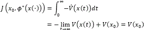
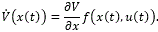
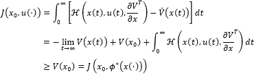
<body><![CDATA[<p align="justify"><font face="verdana" size="2">is predefined&#45;time stable with T(x<sub>0</sub>) &#8804; T<sub>c</sub>. Moreover, the feedback control law <a href="#ec23">(23)</a> minimizes J(x<sub>0</sub>, u(&#8901;)) <a href="#ec18">(18)</a> in the sense that</font></p>  	    <p align="justify"><a name="ec25"/><img src="/img/revistas/eac/v38n1/e2508117.gif">  	    <p align="justify"><font face="verdana" size="2"><i>Proof.</i> Applying Lemma 1.1 to the closed&#45;loop system <a href="#ec24">(24)</a>, predefined&#45;time stability with predefined time T<sub>c</sub> follows directly from the conditions <a href="#ec17">(17)</a>&#45;<a href="#ec20">(20)</a>.</font></p>  	    <p align="justify"><font face="verdana" size="2">To prove <a href="#ec25">(25)</a>, let x(t) be a solution of the system <a href="#ec24">(24)</a>. Then,</font></p>  	    <p align="justify"><font face="verdana" size="2"><img src="/img/revistas/eac/v38n1/i0208117.gif"></font></p>  	    <p align="justify"><font face="verdana" size="2">From the above and <a href="#ec21">(21)</a> it follows</font></p>  	    <p align="justify"><font face="verdana" size="2"><img src="/img/revistas/eac/v38n1/i0308117.gif"></font></p>  	    <p align="justify"><font face="verdana" size="2">Hence,</font></p>  	    <p align="justify"><font face="verdana" size="2"><img src="/img/revistas/eac/v38n1/i0408117.gif"></font></p>  	    <p align="justify"><font face="verdana" size="2">Now, let u(&#8901;) &#8712; U(T<sub>c</sub>) and let x(t) be the solution of <a href="#ec12">(12)</a>, so that</font></p>  	    ]]></body>
<body><![CDATA[<p align="justify"><font face="verdana" size="2"><img src="/img/revistas/eac/v38n1/i0508117.gif"></font></p>  	    <p align="justify"><font face="verdana" size="2">Then,</font></p>  	    <p align="justify"><font face="verdana" size="2"><img src="/img/revistas/eac/v38n1/i0608117.gif"></font></p>  	    <p align="justify"><font face="verdana" size="2">Since u(&#8901;) stabilizes <a href="#ec12">(12)</a> in predefined time T<sub>c</sub>, using <a href="#ec21">(21)</a> and <a href="#ec22">(22)</a> we have</font></p>  	    <p align="justify"><font face="verdana" size="2"><img src="/img/revistas/eac/v38n1/i0708117.gif"></font></p>  	    <p align="justify"><font face="verdana" size="2"><i>Remark 3.1.</i> It is important that the optimal predefined&#45;time stabilizing controller u<sup>*</sup>=&#981;<sup>*</sup>(x) characterized by Theorem 3.1 is a feedback controller.</font></p>  	    <p align="justify"><font face="verdana" size="2"><i>Remark 3.2.</i> Note that the conditions <a href="#ec17">(17)</a>&#45;<a href="#ec22">(22)</a> involve a C<sup>1</sup> predefined&#45;time Lyapunov function (see Lemma 1.1) that is also a solution of the steady state Hamilton&#45;Jacobi&#45;Bellman equation <a href="#ec15">(15)</a>. As usual in optimal control theory, these existence conditions are quite restrictive. However, these conditions are very useful to obtain an inverse optimal predefined&#45;time stabilizing controller, for instance, for a class nonlinear affine control systems with relative degree one.&nbsp; This is a typical case in sliding mode control design, and it will be considered in foregoing.</font></p>  	    <p align="justify"><font face="verdana" size="2">To derive a closed&#45;form expression for the controller, the result of Theorem 3.1 is specialized to nonlinear affine control systems of the form</font></p>  	    <p align="justify"><a name="ec26"/><img src="/img/revistas/eac/v38n1/e2608117.gif">  	    <p align="justify"><font face="verdana" size="2">where x &#8712; &#8476;<sup>n</sup> is the system state, u &#8712; &#8476;<sup>m</sup> is the system control input, f: &#8476;<sup>n</sup> &#8594; &#8476;<sup>n</sup> is a nonlinear function with f(0)=0 and B:&#8476;<sup>n</sup> &#8594; &#8476;<sup>n</sup><sup>&times;</sup><sup>m</sup>.</font></p>  	    ]]></body>
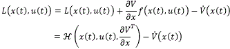
<body><![CDATA[<p align="justify"><font face="verdana" size="2">The performance integrand is also specialized to</font></p>  	    <p align="justify"><a name="ec27"/><img src="/img/revistas/eac/v38n1/e2708117.gif">  	    <p align="justify"><font face="verdana" size="2">where L<sub>1</sub>: &#8476;<sup>n</sup> &#8594; &#8476;, L<sub>2</sub>: &#8476;<sup>n</sup> &#8594; &#8476;<sup>1</sup><sup>&times;</sup><sup>m</sup> and R<sub>2</sub>: &#8476;<sup>n</sup> &#8594; &#8476;<sup>m</sup><sup>&times;</sup><sup>m</sup> is a positive definite matrix function.</font></p>  	    <p align="justify"><font face="verdana" size="2"><i>Theorem 3.2.</i> Assume there exist a C<sup>1</sup> radially unbounded function V: &#8476;<sup>n</sup> &#8594; &#8476;<sub>+</sub> &#8746; {0}, and real numbers T<sub>c</sub> &gt;0 and 0&lt;p&lt; 1 such that</font></p>  	    <p align="justify"><a name="ec28"/><img src="/img/revistas/eac/v38n1/e2808117.gif"> 	    <p align="justify"><a name="ec29"/><img src="/img/revistas/eac/v38n1/e2908117.gif"> 	    <p align="justify"><a name="ec30"/><img src="/img/revistas/eac/v38n1/e3008117.gif"> 	    <p align="justify"><a name="ec31"/><img src="/img/revistas/eac/v38n1/e3108117.gif"> 	    <p align="justify"><a name="ec32"/><img src="/img/revistas/eac/v38n1/e3208117.gif">  	    <p align="justify"><font face="verdana" size="2">Then, with the feedback control</font></p>  	    ]]></body>
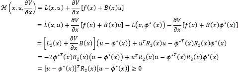
<body><![CDATA[<p align="justify"><a name="ec33"/><img src="/img/revistas/eac/v38n1/e3308117.gif">  	    <p align="justify"><font face="verdana" size="2">the origin of the closed loop system</font></p>  	    <p align="justify"><a name="ec34"/><img src="/img/revistas/eac/v38n1/e3408117.gif">  	    <p align="justify"><font face="verdana" size="2">is predefined&#45;time stable with T(x<sub>0</sub>) &#8804; T<sub>c</sub>. Moreover, the performance measure J(x<sub>0</sub>, u(&#8901;)) is minimized in the sense of <a href="#ec25">(25)</a> and</font></p>  	    <p align="justify"><a name="ec35"/><img src="/img/revistas/eac/v38n1/e3508117.gif">  	    <p align="justify"><font face="verdana" size="2"><i>Proof.</i> Under these conditions the hypotheses of Theorem 3.1 are satisfied. In fact, the control law <a href="#ec33">(33)</a> is obtained solving <img src="/img/revistas/eac/v38n1/i0808117.gif"> =0 with L(x, u) specialized to <a href="#ec27">(27)</a>. Then, setting u<sup>*</sup>=&#981;<sup>*</sup>(x) as in <a href="#ec33">(33)</a>, the conditions <a href="#ec28">(28)</a>, <a href="#ec29">(29)</a> and <a href="#ec30">(30)</a> become the hypotheses <a href="#ec17">(17)</a>, <a href="#ec18">(18)</a> and <a href="#ec20">(20)</a>, respectively.</font></p>  	    <p align="justify"><font face="verdana" size="2">On the other hand, since the function V is C<sup>1</sup>, and by <a href="#ec28">(28)</a>&#45;<a href="#ec29">(29)</a> V has a local minimum at the origin, then <img src="/img/revistas/eac/v38n1/i0908117.gif">=0. Consequently, the hypothesis <a href="#ec19">(19)</a> follows from <a href="#ec31">(31)</a> and the fact that <img src="/img/revistas/eac/v38n1/i0908117.gif">.</font></p>  	    <p align="justify"><font face="verdana" size="2">Since &#981;<sup>*</sup>(x) satisfies <img src="/img/revistas/eac/v38n1/i0808117.gif"><sub>u=&#981;*(x)</sub>=0, and noticing that <a href="#ec23">(23)</a> can be rewritten in terms of &#981;<sup>*</sup>(x) as</font></p>  	    <p align="justify"><a name="ec36"/><img src="/img/revistas/eac/v38n1/e3608117.gif">  	    <p align="justify"><font face="verdana" size="2">then the hypothesis <a href="#ec21">(21)</a> is directly verified.</font></p>  	    ]]></body>
<body><![CDATA[<p align="justify"><font face="verdana" size="2">Finally, from <a href="#ec21">(21)</a>, <a href="#ec33">(33)</a> and the positive definiteness of R<sub>2</sub>(x) it follows</font></p>  	    <p align="justify"><font face="verdana" size="2"><img src="/img/revistas/eac/v38n1/i1008117.gif"></font></p>  	    <p align="justify"><font face="verdana" size="2">which is the hypothesis <a href="#ec22">(22)</a>. Applying Theorem 3.1, the result is obtained.</font></p>  	    <p align="justify"><font face="verdana" size="2"><i>Remark 3.4.</i> The expression <a href="#ec33">(33)</a> provided by Theorem 3.2 can be used to construct an inverse optimal controller, in the following sense: instead of solving the steady&#45;state HJB equation directly to minimize some given performance measure, one can flexibly specify L<sub>2</sub>(x) and R<sub>2</sub>(x), while from <a href="#ec36">(36)</a> L<sub>1</sub>(x) is parameterized as in <a href="#ec36">(36)</a>.</font></p>  	    <p align="justify"><font face="verdana" size="2"><i>Remark 3.5.</i> As in Theorem 3.1, it is not always easy to satisfy the hypotheses <a href="#ec28">(28)</a>&#45;<a href="#ec32">(32)</a> of Theorem 3.2. However, for affine systems with relative degree one, the functions L<sub>2</sub>(x) and R<sub>2</sub>(x) can be chosen such that the conditions <a href="#ec28">(28)</a>&#45;<a href="#ec32">(32)</a> are fulfilled.</font></p>  	    <p align="justify">&nbsp;</p>  	    <p align="justify"><font face="verdana" size="3"><b>4.&#45; INVERSE OPTIMAL PREDEFINED&#45;TIME SLIDING MANIFOLD ReacHING IN LINEAR SYSTEMS.</b></font></p> 	    <p align="justify">&nbsp;</p> 	    <p align="justify"><font face="verdana" size="2"><i>Definition 4.1.</i> &#91;15&#93; Let &#963;: &#8476;<sup>n</sup> &#8594; &#8476;<sup>m</sup> be a smooth function, and define the manifold</font></p>  	    <p align="justify"><a name="ec37"/><img src="/img/revistas/eac/v38n1/e3708117.gif">  	    ]]></body>
<body><![CDATA[<p align="justify"><font face="verdana" size="2">If for an initial condition x<sub>0</sub> &#8712; S, the solution of (1) x(t, x<sub>0</sub>) &#8712; S for all t, the manifold S is called an <i>integral manifold</i>.</font></p>  	    <p align="justify"><font face="verdana" size="2"><i>Definition 4.2.</i> &#91;15&#93; If there is a nonempty set N &#8834; &#8476;<sup>n</sup>&#45;S such that for every initial condition x<sub>0</sub>&#8712; N, there is a finite time t<sub>s</sub> &gt;0 in which the state of the system <a href="#ec1">(1)</a> reaches the manifold S <a href="#ec39">(39)</a>, then the manifold S is called a <i>sliding mode manifold</i>.</font></p>  	    <p align="justify"><font face="verdana" size="2">Consider the following linear time&#45;invariant system subject to perturbation:</font></p>  	    <p align="justify"><a name="ec38"/><img src="/img/revistas/eac/v38n1/e3808117.gif">  	    <p align="justify"><font face="verdana" size="2">where x &#8712; &#8476;<sup>n</sup> is the system state, u &#8712; &#8476;<sup>m</sup>, with m&#8804;n, is the system control input, &#916;: &#8476;<sub>+</sub> &times; &#8476;<sup>n</sup> &#8594; &#8476;<sup>n</sup> is the system perturbation, A &#8712; &#8476;<sup>n</sup><sup>&times;</sup><sup>n</sup>, and B &#8712; &#8476;<sup>n</sup><sup>&times;</sup><sup>m</sup> has full rank.</font></p>  	    <p align="justify"><font face="verdana" size="2">Moreover, consider the function &#963;:&#8476;<sup>n</sup> &#8594; &#8476;<sup>m</sup> as a linear combination of the states</font></p>  	    <p align="justify"><font face="verdana" size="2">&nbsp;&nbsp;&nbsp;&nbsp;&nbsp;&nbsp;&nbsp;&nbsp; &#963;(x)=Sx&nbsp;&nbsp;&nbsp;&nbsp;&nbsp;&nbsp;&nbsp;</font></p>  	    <p align="justify"><font face="verdana" size="2">where S &#8712; &#8476;<sup>m</sup><sup>&times;</sup><sup>n</sup> is full rank.</font></p>  	    <p align="justify"><font face="verdana" size="2">With the above definitions, the main objective of the controller is to optimally drive the trajectories of the system <a href="#ec38">(38)</a> to the set S={x &#8712; &#8476;<sup>n</sup>: Sx=0} <a href="#ec7">(7)</a> in a predefined time in spite of the unknown perturbation &#916;(t, x). The matrix S is selected so that the motion of the system <a href="#ec38">(38)</a> restricted to the sliding manifold &#963;(x)=Sx=0 has a desired behavior.</font></p>  	    <p align="justify"><font face="verdana" size="2">The dynamics of &#963; are described by</font></p>  	    ]]></body>
<body><![CDATA[<p align="justify"><a name="ec39"/><img src="/img/revistas/eac/v38n1/e3908117.gif">  	    <p align="justify"><font face="verdana" size="2">It is assumed that the matrix S is selected such that the square matrix SB &#8712; &#8476;<sup>m&times;m</sup> is nonsingular, i.e., such that the system <a href="#ec39">(39)</a> has relative degree one. This can be easily accomplished since B is full rank.</font></p>  	    <p align="justify"><font face="verdana" size="2"><b>Unperturbed case</b></font></p>  	    <p align="justify"><font face="verdana" size="2">Consider the case when &#916;(t, x)=0. The following result gives an explicit form of the functions V, R<sub>2</sub> and L<sub>2</sub> which characterize the optimal predefined&#45;time stabilizing feedback controller <a href="#ec33">(33)</a>.</font></p>  	    <p align="justify"><font face="verdana" size="2"><i>Corollary 4.1.</i> Consider the system <a href="#ec39">(39)</a> in absence of the perturbation term, i.e., &#916;(t, x)=0. The feedback controller <a href="#ec33">(33)</a> with the functions V, R<sub>2</sub> and L<sub>2</sub> selected as</font></p>  	    <p align="justify"><a name="ec40"/><img src="/img/revistas/eac/v38n1/e4008117.gif"> 	    <p align="justify"><a name="ec41"/><img src="/img/revistas/eac/v38n1/e4108117.gif"> 	    <p align="justify"><a name="ec42"/><img src="/img/revistas/eac/v38n1/e4208117.gif">  	    <p align="justify"><font face="verdana" size="2">with T<sub>c</sub>&gt;0, 0&lt;p&lt;1 and 4c=(p+1)<sup>2</sup>, stabilizes the system <a href="#ec39">(39)</a> in predefined time with sup T(&#963;<sub>0</sub>)=T<sub>c</sub>. Moreover, this controller solves the optimal predefined&#45;time stabilization problem <a href="#ec16">(16)</a> for the system <a href="#ec39">(39)</a> with the performance integrand L(x, u)=L<sub>1</sub>(x)+L<sub>2</sub>(x)u+u<sup>T</sup>R<sub>2</sub>(x)u, where L<sub>2</sub> and R<sub>2</sub> are given by <a href="#ec42">(42)</a> and <a href="#ec41">(41)</a>, respectively, and L<sub>1</sub> is given by <a href="#ec36">(36)</a>.</font></p>  	    <p align="justify"><font face="verdana" size="2"><i>Proof.</i> It is easy to see that all the conditions of Theorem 3.2 are satisfied. Indeed, note that the function V in <a href="#ec40">(40)</a> is C<sup>1</sup>, and satisfies the hypotheses <a href="#ec28">(28)</a> and <a href="#ec29">(29)</a>. In the same manner, the function L<sup>2</sup> in <a href="#ec42">(42)</a> satisfies the hypothesis <a href="#ec31">(31)</a>, and defining the function L<sup>1</sup> as in <a href="#ec36">(36)</a>, the hypothesis <a href="#ec32">(32)</a> is also satisfied.</font></p>  	    ]]></body>
<body><![CDATA[<p align="justify"><font face="verdana" size="2">On the other hand, the derivative of V along <img src="/img/revistas/eac/v38n1/i1108117.gif"> =SAx+SB&#981;<sup>*</sup> is calculated as (note that <img src="/img/revistas/eac/v38n1/i1208117.gif">)</font></p>  	    <p align="justify"><font face="verdana" size="2"><img src="/img/revistas/eac/v38n1/i1208117.gif"></font></p>  	    <p align="justify"><font face="verdana" size="2">Thus, the hypothesis <a href="#ec30">(30)</a> is satisfied. Then, the result is obtained by direct application of Theorem 3.2.</font></p>  	    <p align="justify"><font face="verdana" size="2">&nbsp;</font></p>  	    <p align="justify"><font face="verdana" size="2"><b>Perturbed case</b></font></p>  	    <p align="justify"><font face="verdana" size="2">Now, consider the case when &#916;(t, x) is a matched non&#45;vanishing perturbation. Under the idea of integral sliding mode control &#91;16&#45;17&#93;, the following result provides a controller that rejects the perturbation term &#916;(t, x) in predefined&#45;time and, once the perturbation term is rejected, this controller optimally stabilizes the system <a href="#ec39">(39)</a> in predefined&#45;time.</font></p>  	    <p align="justify"><font face="verdana" size="2"><i>Corollary 4.2.</i> Consider the system <a href="#ec39">(39)</a> and let the function &#916;(t, x) be a matched and non&#45;vanishing perturbation term, i.e. there exists a function <img src="/img/revistas/eac/v38n1/i1408117.gif">(t, x) such that &#916;(t, x)=B<img src="/img/revistas/eac/v38n1/i1408117.gif">(t, x) and &#8214;<img src="/img/revistas/eac/v38n1/i1408117.gif">(t, x)&#8214;&#8804;&#948;, with 0&lt;&#948;&lt;&#8734; a known constant. Then, splitting the control function $u$ into two parts, u=u<sup>0</sup>+u<sup>1</sup>, and selecting</font></p>  	    <p align="justify"><font face="verdana" size="2">(i)&nbsp;&nbsp; u<sub>0</sub> as the optimal predefined&#45;time stabilizing feedback controller <a href="#ec33">(33)</a>, with the functions V, R<sub>2</sub> and L<sub>2</sub> as in Corollary 4.1 with parameters T<sub>c2</sub>&gt;0 and 0&lt;p<sub>2</sub>&lt;1, and</font></p>  	    <p align="justify"><font face="verdana" size="2">(ii)&nbsp; u<sup>1</sup>=&#45;(SB)<sup>&#45;1</sup> &#91;k&#8214;SB&#8214; s/&#8214;s&#8214; + &#934;<sub>p1</sub>(s; T<sub>c1</sub>))&#93;, with T<sub>c1</sub>&gt;0, 0&lt;p<sub>1</sub>&lt;1, k&#8805;&#948;, and the auxiliary sliding variable s=&#963;+z, where z is an integral variable, solution of <img src="/img/revistas/eac/v38n1/i1508117.gif">=&#45;SAx&#45;SBu<sub>0</sub>,</font></p>  	    <p align="justify"><font face="verdana" size="2">the system perturbation term <img src="/img/revistas/eac/v38n1/i1408117.gif">(t, x) is rejected in predefined time T<sub>c1</sub> and, once the perturbation term is rejected, the system <a href="#ec39">(39)</a> is optimally predefined&#45;time stabilized with predefined time T(&#963;<sub>0</sub>) &#8804;T<sub>c2</sub>, with respect to the performance L(x, u)=L<sub>1</sub>(x)+L<sub>2</sub>(x)u+u<sup>T</sup>R<sub>2</sub>(x)u, where L<sub>2</sub> and R<sub>2</sub> are given by <a href="#ec42">(42)</a> and <a href="#ec41">(41)</a>, respectively, and L<sub>1</sub> is given by <a href="#ec36">(36)</a>.</font></p>  	    ]]></body>
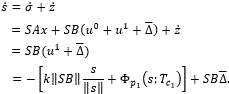
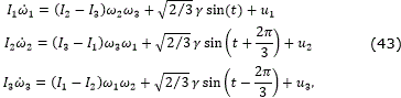
<body><![CDATA[<p align="justify"><font face="verdana" size="2"><i>Proof.</i> By the definition of s, &#963;, z and u<sup>1</sup>, the dynamics of s are obtained as</font></p>  	    <p align="justify"><font face="verdana" size="2"><img src="/img/revistas/eac/v38n1/i1608117.gif"></font></p>  	    <p align="justify"><font face="verdana" size="2">By direct application of Lemma 1.3, s=0 for t&gt;T<sub>c1</sub>. Once the dynamics of <a href="#ec39">(39)</a> are constrained to the manifold s=0, then, from s=0, the equivalent control <a href="#ec3">(3)</a> value of u1 is u<sup>1</sup><sub>eq</sub>=&#45;<img src="/img/revistas/eac/v38n1/i1408117.gif">. Therefore, the sliding mode dynamics of &#963;, <img src="/img/revistas/eac/v38n1/i1108117.gif">=SAx+SBu<sup>0</sup>, are invariant with respect to the perturbation. By the definition of u<sup>0</sup> a direct application of Corollary 4.1 yields the desired result.</font></p>  	    <p align="justify">&nbsp;</p>  	    <p align="justify"><font face="verdana" size="3"><b>5.&#45; EXAMPLE</b></font></p> 	    <p align="justify">&nbsp;</p> 	    <p align="justify"><font face="verdana" size="2">Consider a satellite system as presented in &#91;18&#93;, subject to external disturbances</font></p>  	    <p align="justify"><a name="ec43"/><img src="/img/revistas/eac/v38n1/e4308117.gif">  	    <p align="justify"><font face="verdana" size="2">where, for i=1,2,3; &#969;<sub>i</sub> are the angular velocities of the satellite around the principal axes, u<sub>i</sub> are the control input torques, and I<sub>i</sub> represent the moments of inertia.</font></p>  	    <p align="justify"><font face="verdana" size="2">Defining x<sub>i</sub>=&#969;<sub>i</sub> for i=1,2,3; x=&#91;x<sub>1</sub> x<sub>2</sub> x<sub>3</sub>&#93;<sup>T</sup>, and u=&#91;u<sub>1</sub> u<sub>2</sub> u<sub>3</sub>&#93;<sup>T</sup>, the system <a href="#ec43">(43)</a> can be represented as the linear perturbed system</font></p>  	    ]]></body>
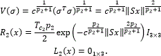
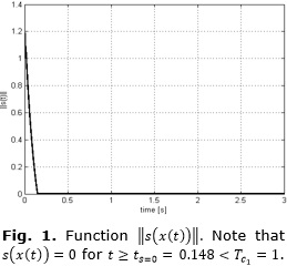
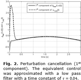
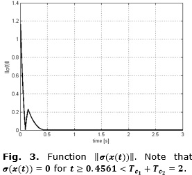
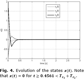
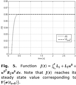
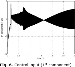
<body><![CDATA[<p align="justify"><font face="verdana" size="2"><img src="/img/revistas/eac/v38n1/i1708117.gif"></font></p>  	    <p align="justify"><font face="verdana" size="2">where &#916;(t, x)=B<img src="/img/revistas/eac/v38n1/i1408117.gif">(t, x) is a matched perturbation which represents the nonlinearities and uncertainties, with B=diag(1/I<sub>1</sub>, 1/I<sub>2</sub>, 1/I<sub>3</sub>), and <img src="/img/revistas/eac/v38n1/i1408117.gif">(t, x)=&#91;(I<sub>2</sub> &#45; I<sub>3</sub>)x<sub>2</sub>x<sub>3</sub>+&#8730;(2&#8260;3)&#947;&middot;sin(t)&middot;(I<sub>3</sub> &#45; I<sub>1</sub>)x<sub>3</sub>x<sub>1</sub> + &#8730;(2&#8260;3)&#947;&middot;sin(t+2&#960;/3)&middot;(I<sub>1</sub> &#45; I<sub>2</sub>)x<sub>1</sub>x<sub>2</sub> + &#8730;(2&#8260;3)&#947;&middot;sin(t&#45;2&#960;/3)&#93;<sup>T</sup>. Furthermore &#8214;<img src="/img/revistas/eac/v38n1/i1408117.gif">(x)&#8214;&#8804;&#948;+&#947;, with &#948;:=<img src="/img/revistas/eac/v38n1/i1808117.gif"> for &#8214;x&#8214;&#8804;r.</font></p>  	    <p align="justify"><font face="verdana" size="2">The goal is to optimally stabilize the equilibrium point x=0 of the satellite (eliminate rotation movements around the principal axes) in predefined time. With this aim, choose &#963;(x)=Sx, with S=diag(I<sub>1</sub>, I<sub>2</sub>, I<sub>3</sub>) so that SB=I<sub>3&times;3</sub>.</font></p>  	    <p align="justify"><font face="verdana" size="2">According to Corollary 4.2, u<sup>0</sup> is implemented as in <a href="#ec33">(33)</a> with the functions V, R<sub>2</sub> and L<sub>2</sub> selected as</font></p>  	    <p align="justify"><font face="verdana" size="2"><img src="/img/revistas/eac/v38n1/i1908117.gif"></font></p>  	    <p align="justify"><font face="verdana" size="2">On the other hand, z and u<sup>1</sup> are chosen according to the part (ii) of Corollary 4.2.</font></p>  	    <p align="justify"><font face="verdana" size="2">Simulations were conducted using the Euler integration method, with a fundamental step size of 1&times;10<sup>&#45;4</sup> s. The numerical values of the parameters are I<sub>1</sub>=1 kg&#8901;m<sup>2</sup>, I<sub>2</sub>=0.8 kg&#8901;m<sup>2</sup>, I<sub>3</sub>=0.4 kg&#8901;m<sup>2</sup> and &#947;=0.5. The initial conditions of the integrators were selected as: x(0)=&#91;0.5 &#45;1&nbsp; 2&#93;<sup>T</sup>, and z(0)=&#91;0&nbsp; 0&nbsp; 0&#93;<sup>T</sup>. In addition, the controller gains were adjusted to: T<sub>c1</sub>=1, T<sub>c2</sub>=1, k=3.9 p<sub>1</sub>=1/3 and p<sub>2</sub>=1/3.</font></p>  	    <p align="justify"><font face="verdana" size="2">Note that s(t)=0 for t&#8805;0.148s:=t<sub>s=0</sub>&lt;T<sub>c1</sub>=1s (see <a href="#fig1">Figure 1</a>), and from that instant on, the equivalent control signal u<sup>1</sup><sub>eq</sub> (approximated using the low&#45;pass filter <img src="/img/revistas/eac/v38n1/i2008117.gif">, &nbsp;with &#964;=0.04, see &#91;3&#93;) cancels the perturbation term <img src="/img/revistas/eac/v38n1/i1408117.gif">(t, x)=&#91;(I<sub>2</sub> &#45; I<sub>3</sub>)x<sub>2</sub>x<sub>3</sub>+&#8730;(2&#8260;3)&#947;&middot;sin(t)&middot;(I<sub>3</sub> &#45; I<sub>1</sub>)x<sub>3</sub>x<sub>1</sub> + &#8730;(2&#8260;3)&#947;&middot;sin(t+2&#960;/3)&middot;(I<sub>1</sub> &#45; I<sub>2</sub>)x<sub>1</sub>x<sub>2</sub> + &#8730;(2&#8260;3)&#947;&middot;sin(t&#45;2&#960;/3)&#93;<sup>T</sup> (see <a href="#fig2">Figure 2</a>).</font></p>  	    <p align="justify"><font face="verdana" size="2">Once the perturbation is canceled, the optimal predefined&#45;time stabilization of the variable &#963;(t) takes place. It can be seen that &#963;(t)=0 for t&#8805;0.4561 s&lt;T<sub>c1</sub>+T<sub>c2</sub>=2s (see <a href="#fig3">Figure 3</a>). It can be noticed that &#963;(x)=Sx=0, if and only if x=0 since S=diag(I<sub>1</sub>, I<sub>2</sub>, I<sub>3</sub>) is invertible. Then, for t&#8805;0.4561s&lt;T<sub>c1</sub>+T<sub>c2</sub>=2s, the state x(t)=0 (see <a href="#fig4">Figure 4</a>).</font></p>  	    <p align="justify"><font face="verdana" size="2"><a href="#fig5">Figure 5</a> shows that the cost, as a function of time, grows quickly to a steady state value corresponding to $V(&#963;(t<sub>s=0</sub>)). Finally, <a href="#fig6">Figure 6</a> shows the first component of the control signal (torque) versus time. It is important to remark that this controller yields discontinuous signals in order to cancel the persistent perturbation <img src="/img/revistas/eac/v38n1/i1408117.gif">(t, x).</font></p>  	    ]]></body>
<body><![CDATA[<p align="center"><a name="fig1"/><img src="/img/revistas/eac/v38n1/f0108117.jpg" width="259" height="240"> 	    <p align="center"><a name="fig2"/><img src="/img/revistas/eac/v38n1/f0208117.jpg" width="267" height="262"> 	    <p align="center"><a name="fig3"/><img src="/img/revistas/eac/v38n1/f0308117.jpg" width="277" height="253"> 	    <p align="center"><a name="fig4"/><img src="/img/revistas/eac/v38n1/f0408117.jpg" width="274" height="255"> 	    <p align="center"><a name="fig5"/><img src="/img/revistas/eac/v38n1/f0508117.jpg" width="267" height="296"> 	    <p align="center"><a name="fig6"/><img src="/img/revistas/eac/v38n1/f0608117.jpg" width="262" height="234"> 	    <p align="justify"><font face="verdana" size="2"><b>&nbsp;</b></font></p>  	    <p align="justify"><font face="verdana" size="3"><b>6.&#45; CONCLUSIONS</b></font></p> 	    <p align="justify">&nbsp;</p> 	    <p align="justify"><font face="verdana" size="2">In this paper, the problem of optimal predefined&#45;time stability was investigated. Sufficient conditions for a controller to be optimal predefined&#45;time stabilizing for a given nonlinear system were provided. Moreover, under the idea of inverse optimal control, and considering nonlinear affine systems and a certain class of performance integrand, the explicit form of the controller was also derived. This class of controllers was applied to the predefined&#45;time optimization of the sliding manifold reaching phase in linear systems, considering both the unperturbed and the perturbed cases. For the unperturbed case, the developed result was applied directly, while for the perturbed case it was used jointly with the idea of integral sliding mode control to provide robustness. The developed control schemes were performed for the predefined&#45;time optimization of the sliding manifold reaching phase in a satellite system model. Simulation results supported the expected results.</font></p>  	    ]]></body>
<body><![CDATA[<p align="justify">&nbsp;</p> 	    <p align="justify"><font face="verdana" size="3"><strong>REFERENCES</strong></font></p> 	    <p align="justify">&nbsp;</p> 	    <!-- ref --><p align="justify"><font face="verdana" size="2">1. &nbsp;&nbsp;&nbsp;&nbsp;&nbsp; Roxin E. On finite stability in control systems. Rend del Circ Mat di Palermo. 1966;15(3):273&#150;82.    </font></p>  	    <!-- ref --><p align="justify"><font face="verdana" size="2">2. &nbsp;&nbsp;&nbsp;&nbsp;&nbsp; Haimo V. Finite Time Controllers. SIAM J Control Optim. 1986;24(4):760&#150;70.    </font></p>  	     <!-- ref --><p align="justify"><font face="verdana" size="2">3. &nbsp;&nbsp;&nbsp;&nbsp;&nbsp;    Utkin VI. Sliding Modes in Control and Optimization. New York: Sciences; 1992.    p. 286.    </font></p>  	    <!-- ref --><p align="justify"><font face="verdana" size="2">4. &nbsp;&nbsp;&nbsp;&nbsp;&nbsp; Bhat S, Bernstein D. Finite&#45;Time Stability of Continuous Autonomous Systems. SIAM J Control Optim. 2000;38(3):751&#150;66.    </font></p>  	     <!-- ref --><p align="justify"><font face="verdana" size="2">5. &nbsp;&nbsp;&nbsp;&nbsp;&nbsp;    Moulay E, Perruquetti W. Finite&#45;Time Stability and Stabilization: State    of the Art. In: Edwards C, Fossas Colet E, Fridman L, editors. Advances in Variable    Structure and Sliding Mode Control. Berlin: Springer Berlin Heidelberg; 2006.    p. 23&#150;41.    </font></p>  	    <!-- ref --><p align="justify"><font face="verdana" size="2">6. &nbsp;&nbsp;&nbsp;&nbsp;&nbsp; Andrieu V, Praly L, Astolfi A. Homogeneous Approximation, Recursive Observer Design, and Output Feedback. SIAM J Control Optim. 2008;47(4):1814&#150;50.    </font></p>  	     <!-- ref --><p align="justify"><font face="verdana" size="2">7. &nbsp;&nbsp;&nbsp;&nbsp;&nbsp;    Cruz&#45;Zavala E, Moreno JA, Fridman L. Uniform Second&#45;Order Sliding Mode    Observer for mechanical systems. In: Proceedings of the 2010 11th International    Workshop on Variable Structure Systems (VSS 2010). 2010. p. 14&#150;9.    </font></p>  	    <!-- ref --><p align="justify"><font face="verdana" size="2">8. &nbsp;&nbsp;&nbsp;&nbsp;&nbsp; Polyakov A. Nonlinear Feedback Design for Fixed&#45;Time Stabilization of Linear Control Systems. IEEE Trans Automat Contr. 2012;57(8):2106&#150;10.    </font></p>  	    <!-- ref --><p align="justify"><font face="verdana" size="2">9. &nbsp;&nbsp;&nbsp;&nbsp;&nbsp; Polyakov A, Fridman L. Stability notions and {L}yapunov functions for sliding mode control systems. J Franklin Inst. 2014;351(4):1831&#150;65.    </font></p>  	     <!-- ref --><p align="justify"><font face="verdana" size="2">10. &nbsp;&nbsp;&nbsp; S&aacute;nchez&#45;Torres    JD, S&aacute;nchez EN, Loukianov AG. A discontinuous recurrent neural network    with predefined time convergence for solution of linear programming. In: IEEE    Symposium on Swarm Intelligence (SIS). 2014. p. 9&#150;12.    </font></p>  	     <!-- ref --><p align="justify"><font face="verdana" size="2">11. &nbsp;&nbsp;&nbsp; S&aacute;nchez&#45;Torres    JD, Sanchez EN, Loukianov AG. Predefined&#45;time stability of dynamical systems    with sliding modes. In: American Control Conference (ACC) 2015. 2015. p. 5842&#150;6.    </font></p>  	    <!-- ref --><p align="justify"><font face="verdana" size="2">12. &nbsp;&nbsp;&nbsp; Bernstein DS. Nonquadratic Cost and Nonlinear Feedback Control. Int J Robust Nonlinear Control. 1993;3(1):211&#150;29.    </font></p>  	     <!-- ref --><p align="justify"><font face="verdana" size="2">13. &nbsp;&nbsp;&nbsp; Haddad    WM, L&#8217;Afflitto A. Finite&#45;Time Stabilization and Optimal Feedback Control.    IEEE Trans Automat Contr. 2016;61(4):1069&#150;74.    </font></p>  	     <!-- ref --><p align="justify"><font face="verdana" size="2">14. &nbsp;&nbsp;&nbsp; Jim&eacute;nez&#45;Rodr&iacute;guez    E, S&aacute;nchez&#45;Torres JD, Loukianov AG. On Optimal Predefined&#45;Time    Stabilization. In: Proceedings of the XVII Latin American Conference in Automatic    Control. 2016. p. 317&#150;22.    </font></p>  	     <!-- ref --><p align="justify"><font face="verdana" size="2">15. &nbsp;&nbsp;&nbsp; Drakunov    S V., Utkin VI. Sliding mode control in dynamic systems. International Journal    of Control. 1992; 55(4): 1029&#150;37.    </font></p>  	    <!-- ref --><p align="justify"><font face="verdana" size="2">16. &nbsp;&nbsp;&nbsp; Matthews GP, DeCarlo RA. Decentralized tracking for a class of interconnected nonlinear systems using variable structure control. Automatica. 1988;24(2):187&#150;93.    </font></p>  	     <!-- ref --><p align="justify"><font face="verdana" size="2">17. &nbsp;&nbsp;&nbsp; Utkin    VI, Shi J. Integral sliding mode in systems operating under uncertainty conditions.    In: Proc 35th IEEE Conf Decis Control. 1996. p. 4.    </font></p>  	    <!-- ref --><p align="justify"><font face="verdana" size="2">18. &nbsp;&nbsp;&nbsp; Shtessel Y, Edwards C, Fridman L, Levant A. Sliding Mode Control and Observation. New York: Springer; 2014.    </font></p>  	    <p align="justify">&nbsp;</p>     ]]></body>
<body><![CDATA[<p align="justify">&nbsp;</p>     <p align="justify"><font face="verdana" size="2">Received: 15 de septiembre del    2016&nbsp;&nbsp;&nbsp;&nbsp;&nbsp;&nbsp;    <br>   Approved: 8 de enero del 2017</font></p>     <p align="justify">&nbsp;</p>     <p align="justify">&nbsp;</p>  	    <p align="justify"><font face="verdana" size="2"><i>Esteban Jim&eacute;nez Rodr&iacute;guez</i>, Advanced Studies and Research Center of the National Polytechnic Institute &#45;CINVESTAV&#45;, Campus Guadalajara, M&eacute;xico. E&#45;mail: <a href="mailto:esjimenezro@gmail.com">esjimenezro@gmail.com</a>.</font></p>       ]]></body><back>
<ref-list>
<ref id="B1">
<label>1</label><nlm-citation citation-type="journal">
<person-group person-group-type="author">
<name>
<surname><![CDATA[Roxin]]></surname>
<given-names><![CDATA[E]]></given-names>
</name>
</person-group>
<article-title xml:lang="en"><![CDATA[On finite stability in control systems]]></article-title>
<source><![CDATA[Rend del Circ Mat di Palermo]]></source>
<year>1966</year>
<volume>15</volume>
<numero>3</numero>
<issue>3</issue>
<page-range>273-82</page-range></nlm-citation>
</ref>
<ref id="B2">
<label>2</label><nlm-citation citation-type="journal">
<person-group person-group-type="author">
<name>
<surname><![CDATA[Haimo]]></surname>
<given-names><![CDATA[V]]></given-names>
</name>
</person-group>
<article-title xml:lang="en"><![CDATA[Finite Time Controllers]]></article-title>
<source><![CDATA[SIAM J Control Optim]]></source>
<year>1986</year>
<volume>24</volume>
<numero>4</numero>
<issue>4</issue>
<page-range>760-70</page-range></nlm-citation>
</ref>
<ref id="B3">
<label>3</label><nlm-citation citation-type="book">
<person-group person-group-type="author">
<name>
<surname><![CDATA[Utkin]]></surname>
<given-names><![CDATA[VI]]></given-names>
</name>
</person-group>
<source><![CDATA[Sliding Modes in Control and Optimization]]></source>
<year>1992</year>
<page-range>286</page-range><publisher-loc><![CDATA[New York ]]></publisher-loc>
<publisher-name><![CDATA[Sciences]]></publisher-name>
</nlm-citation>
</ref>
<ref id="B4">
<label>4</label><nlm-citation citation-type="journal">
<person-group person-group-type="author">
<name>
<surname><![CDATA[Bhat]]></surname>
<given-names><![CDATA[S]]></given-names>
</name>
<name>
<surname><![CDATA[Bernstein]]></surname>
<given-names><![CDATA[D]]></given-names>
</name>
</person-group>
<article-title xml:lang="en"><![CDATA[Finite-Time Stability of Continuous Autonomous Systems]]></article-title>
<source><![CDATA[SIAM J Control Optim]]></source>
<year>2000</year>
<volume>38</volume>
<numero>3</numero>
<issue>3</issue>
<page-range>751-66</page-range></nlm-citation>
</ref>
<ref id="B5">
<label>5</label><nlm-citation citation-type="book">
<person-group person-group-type="author">
<name>
<surname><![CDATA[Moulay]]></surname>
<given-names><![CDATA[E]]></given-names>
</name>
<name>
<surname><![CDATA[Perruquetti]]></surname>
<given-names><![CDATA[W]]></given-names>
</name>
</person-group>
<article-title xml:lang="en"><![CDATA[Finite-Time Stability and Stabilization: State of the Art]]></article-title>
<person-group person-group-type="editor">
<name>
<surname><![CDATA[Edwards]]></surname>
<given-names><![CDATA[C]]></given-names>
</name>
<name>
<surname><![CDATA[Fossas Colet]]></surname>
<given-names><![CDATA[E]]></given-names>
</name>
<name>
<surname><![CDATA[Fridman]]></surname>
<given-names><![CDATA[L]]></given-names>
</name>
</person-group>
<source><![CDATA[Advances in Variable Structure and Sliding Mode Control]]></source>
<year>2006</year>
<page-range>23-41</page-range><publisher-loc><![CDATA[Berlin ]]></publisher-loc>
<publisher-name><![CDATA[Springer Berlin Heidelberg]]></publisher-name>
</nlm-citation>
</ref>
<ref id="B6">
<label>6</label><nlm-citation citation-type="journal">
<person-group person-group-type="author">
<name>
<surname><![CDATA[Andrieu]]></surname>
<given-names><![CDATA[V]]></given-names>
</name>
<name>
<surname><![CDATA[Praly]]></surname>
<given-names><![CDATA[L]]></given-names>
</name>
<name>
<surname><![CDATA[Astolfi]]></surname>
<given-names><![CDATA[A]]></given-names>
</name>
</person-group>
<article-title xml:lang="en"><![CDATA[Homogeneous Approximation, Recursive Observer Design, and Output Feedback]]></article-title>
<source><![CDATA[SIAM J Control Optim]]></source>
<year>2008</year>
<volume>47</volume>
<numero>4</numero>
<issue>4</issue>
<page-range>1814-50</page-range></nlm-citation>
</ref>
<ref id="B7">
<label>7</label><nlm-citation citation-type="confpro">
<person-group person-group-type="author">
<name>
<surname><![CDATA[Cruz-Zavala]]></surname>
<given-names><![CDATA[E]]></given-names>
</name>
<name>
<surname><![CDATA[Moreno]]></surname>
<given-names><![CDATA[JA]]></given-names>
</name>
<name>
<surname><![CDATA[Fridman]]></surname>
<given-names><![CDATA[L]]></given-names>
</name>
</person-group>
<article-title xml:lang="en"><![CDATA[Uniform Second-Order Sliding Mode Observer for mechanical systems]]></article-title>
<source><![CDATA[]]></source>
<year>2010</year>
<conf-name><![CDATA[11 International Workshop on Variable Structure Systems]]></conf-name>
<conf-date>2010</conf-date>
<conf-loc> </conf-loc>
<page-range>14-9</page-range></nlm-citation>
</ref>
<ref id="B8">
<label>8</label><nlm-citation citation-type="journal">
<person-group person-group-type="author">
<name>
<surname><![CDATA[Polyakov]]></surname>
<given-names><![CDATA[A]]></given-names>
</name>
</person-group>
<article-title xml:lang="en"><![CDATA[Nonlinear Feedback Design for Fixed-Time Stabilization of Linear Control Systems]]></article-title>
<source><![CDATA[IEEE Trans Automat Contr]]></source>
<year>2012</year>
<volume>57</volume>
<numero>8</numero>
<issue>8</issue>
<page-range>2106-10</page-range></nlm-citation>
</ref>
<ref id="B9">
<label>9</label><nlm-citation citation-type="journal">
<person-group person-group-type="author">
<name>
<surname><![CDATA[Polyakov]]></surname>
<given-names><![CDATA[A]]></given-names>
</name>
<name>
<surname><![CDATA[Fridman]]></surname>
<given-names><![CDATA[L]]></given-names>
</name>
</person-group>
<article-title xml:lang="en"><![CDATA[Stability notions and {L}yapunov functions for sliding mode control systems]]></article-title>
<source><![CDATA[J Franklin Inst]]></source>
<year>2014</year>
<volume>351</volume>
<numero>4</numero>
<issue>4</issue>
<page-range>1831-65</page-range></nlm-citation>
</ref>
<ref id="B10">
<label>10</label><nlm-citation citation-type="confpro">
<person-group person-group-type="author">
<name>
<surname><![CDATA[Sánchez-Torres]]></surname>
<given-names><![CDATA[JD]]></given-names>
</name>
<name>
<surname><![CDATA[Sánchez]]></surname>
<given-names><![CDATA[EN]]></given-names>
</name>
<name>
<surname><![CDATA[Loukianov]]></surname>
<given-names><![CDATA[AG]]></given-names>
</name>
</person-group>
<source><![CDATA[A discontinuous recurrent neural network with predefined time convergence for solution of linear programming]]></source>
<year>2014</year>
<conf-name><![CDATA[ IEEE Symposium on Swarm Intelligence]]></conf-name>
<conf-loc> </conf-loc>
<page-range>9-12</page-range></nlm-citation>
</ref>
<ref id="B11">
<label>11</label><nlm-citation citation-type="confpro">
<person-group person-group-type="author">
<name>
<surname><![CDATA[Sánchez-Torres]]></surname>
<given-names><![CDATA[JD]]></given-names>
</name>
<name>
<surname><![CDATA[Sanchez]]></surname>
<given-names><![CDATA[EN]]></given-names>
</name>
<name>
<surname><![CDATA[Loukianov]]></surname>
<given-names><![CDATA[AG]]></given-names>
</name>
</person-group>
<source><![CDATA[Predefined-time stability of dynamical systems with sliding modes]]></source>
<year>2015</year>
<conf-name><![CDATA[ American Control Conference]]></conf-name>
<conf-date>2015</conf-date>
<conf-loc> </conf-loc>
<page-range>5842-6</page-range></nlm-citation>
</ref>
<ref id="B12">
<label>12</label><nlm-citation citation-type="journal">
<person-group person-group-type="author">
<name>
<surname><![CDATA[Bernstein]]></surname>
<given-names><![CDATA[DS]]></given-names>
</name>
</person-group>
<article-title xml:lang="en"><![CDATA[Nonquadratic Cost and Nonlinear Feedback Control]]></article-title>
<source><![CDATA[Int J Robust Nonlinear Control]]></source>
<year>1993</year>
<volume>3</volume>
<numero>1</numero>
<issue>1</issue>
<page-range>211-29</page-range></nlm-citation>
</ref>
<ref id="B13">
<label>13</label><nlm-citation citation-type="journal">
<person-group person-group-type="author">
<name>
<surname><![CDATA[Haddad]]></surname>
<given-names><![CDATA[WM]]></given-names>
</name>
</person-group>
<collab>L'Afflitto A</collab>
<article-title xml:lang="en"><![CDATA[Finite-Time Stabilization and Optimal Feedback Control]]></article-title>
<source><![CDATA[IEEE Trans Automat Contr]]></source>
<year>2016</year>
<volume>61</volume>
<numero>4</numero>
<issue>4</issue>
<page-range>1069-74</page-range></nlm-citation>
</ref>
<ref id="B14">
<label>14</label><nlm-citation citation-type="confpro">
<person-group person-group-type="author">
<name>
<surname><![CDATA[Jiménez-Rodríguez]]></surname>
<given-names><![CDATA[E]]></given-names>
</name>
<name>
<surname><![CDATA[Sánchez-Torres]]></surname>
<given-names><![CDATA[JD]]></given-names>
</name>
<name>
<surname><![CDATA[Loukianov]]></surname>
<given-names><![CDATA[AG]]></given-names>
</name>
</person-group>
<source><![CDATA[On Optimal Predefined-Time Stabilization]]></source>
<year>2016</year>
<conf-name><![CDATA[XVII Latin American Conference in Automatic Control]]></conf-name>
<conf-loc> </conf-loc>
<page-range>317-22</page-range></nlm-citation>
</ref>
<ref id="B15">
<label>15</label><nlm-citation citation-type="journal">
<person-group person-group-type="author">
<name>
<surname><![CDATA[Drakunov]]></surname>
<given-names><![CDATA[SV]]></given-names>
</name>
<name>
<surname><![CDATA[Utkin]]></surname>
<given-names><![CDATA[VI]]></given-names>
</name>
</person-group>
<article-title xml:lang="en"><![CDATA[Sliding mode control in dynamic systems]]></article-title>
<source><![CDATA[International Journal of Control]]></source>
<year>1992</year>
<volume>55</volume>
<numero>4</numero>
<issue>4</issue>
<page-range>1029-37</page-range></nlm-citation>
</ref>
<ref id="B16">
<label>16</label><nlm-citation citation-type="journal">
<person-group person-group-type="author">
<name>
<surname><![CDATA[Matthews]]></surname>
<given-names><![CDATA[GP]]></given-names>
</name>
<name>
<surname><![CDATA[DeCarlo]]></surname>
<given-names><![CDATA[RA]]></given-names>
</name>
</person-group>
<article-title xml:lang="en"><![CDATA[Decentralized tracking for a class of interconnected nonlinear systems using variable structure control]]></article-title>
<source><![CDATA[Automatica]]></source>
<year>1988</year>
<volume>24</volume>
<numero>2</numero>
<issue>2</issue>
<page-range>187-93</page-range></nlm-citation>
</ref>
<ref id="B17">
<label>17</label><nlm-citation citation-type="confpro">
<person-group person-group-type="author">
<name>
<surname><![CDATA[Utkin]]></surname>
<given-names><![CDATA[VI]]></given-names>
</name>
<name>
<surname><![CDATA[Shi]]></surname>
<given-names><![CDATA[J]]></given-names>
</name>
</person-group>
<source><![CDATA[Integral sliding mode in systems operating under uncertainty conditions]]></source>
<year>1996</year>
<conf-name><![CDATA[35 IEEE Conf Decis Control]]></conf-name>
<conf-loc> </conf-loc>
<page-range>4</page-range></nlm-citation>
</ref>
<ref id="B18">
<label>18</label><nlm-citation citation-type="book">
<person-group person-group-type="author">
<name>
<surname><![CDATA[Shtessel]]></surname>
<given-names><![CDATA[Y]]></given-names>
</name>
<name>
<surname><![CDATA[Edwards]]></surname>
<given-names><![CDATA[C]]></given-names>
</name>
<name>
<surname><![CDATA[Fridman]]></surname>
<given-names><![CDATA[L]]></given-names>
</name>
<name>
<surname><![CDATA[Levant]]></surname>
<given-names><![CDATA[A]]></given-names>
</name>
</person-group>
<source><![CDATA[Sliding Mode Control and Observation]]></source>
<year>2014</year>
<publisher-loc><![CDATA[New York ]]></publisher-loc>
<publisher-name><![CDATA[Springer]]></publisher-name>
</nlm-citation>
</ref>
</ref-list>
</back>
</article>