<?xml version="1.0" encoding="ISO-8859-1"?><article xmlns:mml="http://www.w3.org/1998/Math/MathML" xmlns:xlink="http://www.w3.org/1999/xlink" xmlns:xsi="http://www.w3.org/2001/XMLSchema-instance">
<front>
<journal-meta>
<journal-id>1815-5928</journal-id>
<journal-title><![CDATA[Ingeniería Electrónica, Automática y Comunicaciones]]></journal-title>
<abbrev-journal-title><![CDATA[EAC]]></abbrev-journal-title>
<issn>1815-5928</issn>
<publisher>
<publisher-name><![CDATA[Universidad Tecnológica de La Habana José Antonio Echeverría, Cujae]]></publisher-name>
</publisher>
</journal-meta>
<article-meta>
<article-id>S1815-59282017000100007</article-id>
<title-group>
<article-title xml:lang="en"><![CDATA[Neural Control for Photovoltaic Panel Maximum Power Point Tracking]]></article-title>
<article-title xml:lang="es"><![CDATA[Control Neuronal para el Seguimiento del Máximo Punto de Potencia de un Panel Fotovoltaico]]></article-title>
</title-group>
<contrib-group>
<contrib contrib-type="author">
<name>
<surname><![CDATA[Loza-López]]></surname>
<given-names><![CDATA[Martin J.]]></given-names>
</name>
<xref ref-type="aff" rid="A01"/>
</contrib>
<contrib contrib-type="author">
<name>
<surname><![CDATA[López-García]]></surname>
<given-names><![CDATA[Tania B.]]></given-names>
</name>
<xref ref-type="aff" rid="A01"/>
</contrib>
<contrib contrib-type="author">
<name>
<surname><![CDATA[Ruíz-Cruz]]></surname>
<given-names><![CDATA[Riemann]]></given-names>
</name>
<xref ref-type="aff" rid="A01"/>
</contrib>
<contrib contrib-type="author">
<name>
<surname><![CDATA[Sánchez]]></surname>
<given-names><![CDATA[Edgar N.]]></given-names>
</name>
<xref ref-type="aff" rid="A01"/>
</contrib>
</contrib-group>
<aff id="A01">
<institution><![CDATA[,Centro de Investigación y Estudios Avanzados del Instituto Politécnico Nacional  ]]></institution>
<addr-line><![CDATA[Jalisco ]]></addr-line>
<country>Mexico</country>
</aff>
<pub-date pub-type="pub">
<day>00</day>
<month>04</month>
<year>2017</year>
</pub-date>
<pub-date pub-type="epub">
<day>00</day>
<month>04</month>
<year>2017</year>
</pub-date>
<volume>38</volume>
<numero>1</numero>
<fpage>79</fpage>
<lpage>89</lpage>
<copyright-statement/>
<copyright-year/>
<self-uri xlink:href="http://scielo.sld.cu/scielo.php?script=sci_arttext&amp;pid=S1815-59282017000100007&amp;lng=en&amp;nrm=iso"></self-uri><self-uri xlink:href="http://scielo.sld.cu/scielo.php?script=sci_abstract&amp;pid=S1815-59282017000100007&amp;lng=en&amp;nrm=iso"></self-uri><self-uri xlink:href="http://scielo.sld.cu/scielo.php?script=sci_pdf&amp;pid=S1815-59282017000100007&amp;lng=en&amp;nrm=iso"></self-uri><abstract abstract-type="short" xml:lang="en"><p><![CDATA[With the rise in the use of renewable energies, solar panels have proven to be reliable and have a favorable cost-benefit ratio, producing energy free of noise and air pollution. Solar panels are subject to considerable variations in working conditions due to changes in solar irradiation levels and temperature that affect its semiconductor properties. To be able to profit as much as possible from this source of energy, control of the modules and perturbation rejection is very important to obtain the highest viable amount of electrical power. This work is concerned with the on-line identification and control of a photovoltaic system using neural networks with the Kalman Filter as training algorithm. Having on-line identification and control allows the system to be more adaptable to changes in weather and other variations than with common off-line methods.]]></p></abstract>
<abstract abstract-type="short" xml:lang="es"><p><![CDATA[Dado el aumento en el uso de energía renovable, los paneles solares han demostrado ser de confianza y tener una proporción costo-beneficio favorable, produciendo energía libre de ruido y contaminación del aire. Los paneles solares están sujetos a variaciones considerables en sus condiciones de trabajo debido a cambios en niveles de irradiación solar y en temperatura, esto afecta sus propiedades como semiconductor. Para poder aprovechar lo más posible esta fuente de energía, control de los módulos y rechazo a perturbaciones es muy importante para obtener la máxima cantidad disponible de poder eléctrico. Este trabajo está centrado en la identificación y el control en-línea de un sistema fotovoltaico, usando redes neuronales con el filtro de Kalman como algoritmo de entrenamiento. Al tener identificación y control en-línea, el sistema se vuelve más adaptable a cambios en el clima y a otras variaciones en comparación con métodos fuera de línea que son más comunes.]]></p></abstract>
<kwd-group>
<kwd lng="en"><![CDATA[Photovoltaic systems]]></kwd>
<kwd lng="en"><![CDATA[solar energy]]></kwd>
<kwd lng="en"><![CDATA[high order neural networks]]></kwd>
<kwd lng="en"><![CDATA[Kalman filter]]></kwd>
<kwd lng="en"><![CDATA[maximum power point tracking]]></kwd>
<kwd lng="es"><![CDATA[Sistemas fotovoltaicos]]></kwd>
<kwd lng="es"><![CDATA[energía solar]]></kwd>
<kwd lng="es"><![CDATA[redes neuronales de alto orden]]></kwd>
<kwd lng="es"><![CDATA[filtro de Kalman]]></kwd>
<kwd lng="es"><![CDATA[seguimiento del punto de máxima potencia]]></kwd>
</kwd-group>
</article-meta>
</front><body><![CDATA[  	    <p align="right"><font face="Verdana" size="2"> <b>ORIGINAL ARTICLE</b></font></p>     <p align="justify">&nbsp;</p>     <p align="justify">&nbsp; </p> 	    <p align="justify"><strong><font face="verdana" size="4">Neural Control for Photovoltaic Panel Maximum Power Point Tracking</font></strong></p> 	    <p align="justify">&nbsp;</p> 	    <p align="justify"><font face="verdana" size="3"><b>Control Neuronal para el Seguimiento del M&aacute;ximo Punto de Potencia de un Panel Fotovoltaico</b></font></p>  	    <p align="justify">&nbsp;</p> 	    <p align="justify">&nbsp;</p> 	     <p align="justify"><font face="verdana" size="2"><b>Martin J. Loza&#45;L&oacute;pez,    Tania B. L&oacute;pez&#45;Garc&iacute;a, Riemann Ru&iacute;z&#45;Cruz, Edgar    N. S&aacute;nchez</b></font></p> 	    ]]></body>
<body><![CDATA[<p align="justify"><font face="verdana" size="2">Centro de Investigaci&oacute;n y Estudios Avanzados del Instituto Polit&eacute;cnico Nacional, Jalisco, Mexico.</font></p> 	    <p align="justify">&nbsp;</p>     <p align="justify">&nbsp;</p> <hr align="JUSTIFY" size="1" noshade>  	    <p align="justify"><font face="verdana" size="2"><strong>ABSTRACT</strong></font></p>  	     <p align="justify"><font face="verdana" size="2">With the rise in the use of renewable    energies, solar panels have proven to be reliable and have a favorable cost&#45;benefit    ratio, producing energy free of noise and air pollution. Solar panels are subject    to considerable variations in working conditions due to changes in solar irradiation    levels and temperature that affect its semiconductor properties. To be able    to profit as much as possible from this source of energy, control of the modules    and perturbation rejection is very important to obtain the highest viable amount    of electrical power. This work is concerned with the on&#45;line identification    and control of a photovoltaic system using neural networks with the Kalman Filter    as training algorithm. Having on&#45;line identification and control allows    the system to be more adaptable to changes in weather and other variations than    with common off&#45;line methods.</font></p>  	     <p align="justify"><font face="verdana" size="2"><b>Keywords:</b> Photovoltaic    systems, solar energy, high order neural networks, Kalman filter, maximum power    point tracking.</font></p>  	<hr align="JUSTIFY" size="1" noshade>     <p align="justify"><font face="verdana" size="2"><b>RESUMEN</b></font></p>  	     <p align="justify"><font face="verdana" size="2">Dado el aumento en el uso de    energ&iacute;a renovable, los paneles solares han demostrado ser de confianza    y tener una proporci&oacute;n costo&#45;beneficio favorable, produciendo energ&iacute;a    libre de ruido y contaminaci&oacute;n del aire. Los paneles solares est&aacute;n    sujetos a variaciones considerables en sus condiciones de trabajo debido a cambios    en niveles de irradiaci&oacute;n solar y en temperatura, esto afecta sus propiedades    como semiconductor. Para poder aprovechar lo m&aacute;s posible esta fuente    de energ&iacute;a, control de los m&oacute;dulos y rechazo a perturbaciones    es muy importante para obtener la m&aacute;xima cantidad disponible de poder    el&eacute;ctrico. Este trabajo est&aacute; centrado en la identificaci&oacute;n    y el control en&#45;l&iacute;nea de un sistema fotovoltaico, usando redes neuronales    con el filtro de Kalman como algoritmo de entrenamiento. Al tener identificaci&oacute;n    y control en&#45;l&iacute;nea, el sistema se vuelve m&aacute;s adaptable a cambios    en el clima y a otras variaciones en comparaci&oacute;n con m&eacute;todos fuera    de l&iacute;nea que son m&aacute;s comunes.</font></p>  	     <p align="justify"><font face="verdana" size="2"><b>Palabras Claves:</b> Sistemas    fotovoltaicos, energ&iacute;a solar, redes neuronales de alto orden, filtro    de Kalman, seguimiento del punto de m&aacute;xima potencia.</font></p>  	<hr align="JUSTIFY" size="1" noshade>     <p align="justify">&nbsp;</p>     ]]></body>
<body><![CDATA[<p align="justify">&nbsp;</p>     <p align="justify"><font face="verdana" size="3"><b>1.&#45;</b> <b>INTRODUCTION</b></font></p>     <p align="justify">&nbsp;</p>  	    <p align="justify"><font face="verdana" size="2">This work is concerned with the application of recurrent high order neural networks to design a robust photovoltaic panel model and to control the output voltage of the panel (V<sub>PV</sub>) to obtainthe maximum power available.</font></p>  	    <p align="justify"><font face="verdana" size="2">It is important to understand the impact that different uncertainties and parameter variations have on the mathematical model of solar panels, since their efficiency depends greatly on environmental conditions (temperature, solar irradiance, &hellip;). In the field of neural networks there are several studies that focus on the characterization and modeling of solar panels based on artificial intelligence &#91;1&#93;.&nbsp; Another popular use of artificial neural networks is that of designing maximum power point trackers for solar photovoltaic (SPV) modules, as can be observed in &#91;2&#45;4&#93;. The methods usually applied are fuzzy logic controllers, genetic algorithms, and radial basis functions; and most of the time they are off&#45;line methods.</font></p>  	    <p align="justify"><font face="verdana" size="2">In order to solve the problem of time&#45;varying parameters and uncertainties, in this paper the on&#45;line identification and control is proposed. The maximum power point tracker (MPPT) is obtained by means of a searching algorithm; the system is&nbsp;controlled &nbsp;to &nbsp;track &nbsp;the &nbsp;maximum &nbsp;power&nbsp;point &nbsp;using &nbsp;a neural &nbsp;network &nbsp;to &nbsp;identify&nbsp;the &nbsp;model &nbsp;on&#45;line. Afterwards, a</font> <font face="verdana" size="2">controller which regulates the switching frequency of an insulated&#45;gate bipolar transistor (IGBT) in the DC&#45;DC buck converter, based on the identified model, is developed.</font></p>  	     <p align="justify"><font face="verdana" size="2">The advantage of this method    is that the model is not greatly affected by the high frequency noise created    by the IGBT and other perturbations, and so it is possible to reduce the use    of filters. A conventional <i>perturb and observe</i> maximum power point tracker    is used to find the output voltage of the solar panel (V<sub>PV</sub>)necessary    to have the maximum electrical power &#91;5, 6&#93;.</font></p>     <p align="justify"><font face="verdana" size="2">This paper is organized as follows.    In section 2, mathematical preliminaries are given, including a review of photovoltaic    systems, neural networks and the Kalman filter.&nbsp; In section 3, the neural    control is presented, starting with the model of the DC&#45;DC buck converter,    and continuing with the identification and control design. In section 4, the    results are validated using Simulink's Simscape Power Systems Blocks <a name="_ftnref1"></a><a href="#_ftn1"><sup>1</sup></a>,and    a comparison of the neural controller developed with a discrete sliding modes    controller is shown.&nbsp; Finally, in section 5, the conclusions are presented.</font></p> 	    <p align="justify">&nbsp;</p> 	    <p align="justify"><font face="verdana" size="3"><b>2.&#45;MATHEMATICAL PRELIMINARIES</b></font></p> 	    ]]></body>
<body><![CDATA[<p align="justify">&nbsp;</p> 	    <p align="justify"><font face="verdana" size="2"><b>2.1.&#45; MPPT ALGORITHM APPLIEDTO PHOTOVOLTAIC SYSTEMS</b></font></p>  	     <p align="justify"><font face="verdana" size="2">Photovoltaic systems use solar    cells to capture solar energy and convert it into electricity. These systems    are generally made from modified silicon and other semiconductor materials,    they are usually long lasting (25 to 30 years); with the advance of technology    there has been a rise in variety of manufacturers and models available, for    a lower price.</font></p>  	     <p align="justify"><font face="verdana" size="2">Solar panels can be modeled using    an equivalent circuit which consists of a current source I<sub>CC </sub>(whose    value in amperes depends on the irradiance at the moment of measurement), a    diode for discharge, and two resistors; one of them represents losses due to    bad connections (R<sub>s</sub>) and the other represents the leakage current    from the capacitor (R<sub>sh</sub>).&nbsp;The equation that defines the behavior    of said equivalent model is &#91;7&#93;:</font></p>  	    <p align="justify"><a name="ec1"/><img src="/img/revistas/eac/v38n1/e0107117.gif">  	     <p align="justify"><font face="verdana" size="2">where k is the Boltzman constant,    T is the absolute temperature in the photovoltaic panel, I<sub>o</sub> is the    inverse saturation current of the diode, q is the charge of the electron, and    n is the ideality factor of the diode.
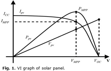
</font></p>  	     <p align="justify"><font face="verdana" size="2">From <a href="#ec1">(1)</a>,    it is clear that there exists a relationship between the voltage and the current    in the photovoltaic panel. This relationship can be observed in <a href="#fig1">Figure    1</a>, which shows the existence of a unique maximum power point P<sub>MPP</sub>,    for each solar panel depending on the temperature and irradiance at the moment    of measurement.</font></p>  	    <p align="center"><a name="fig1"/><img src="/img/revistas/eac/v38n1/f0107117.jpg" width="367" height="237"> 	     <p align="justify"><font face="verdana" size="2">To be able to successfully follow    the maximum power point of the solar panel, it is necessary to have a reference    voltage which corresponds to that point, and to design a controller to track    that reference voltage; this is commonly known as a maximum power point tracker    (MPPT). In the literature, there are several algorithms that have been developed    for this purpose, based on neural networks, incremental conductance, fuzzy logic,    etc., &#91;8&#93;. In this paper, the MPPT algorithm used is known as the <i>perturb</i><i>    and observe</i> method which can be implemented in real&#45;time, and it is    one of the algorithms most commonly used for this purpose. This algorithm is    based on the following criterion: the voltage of the solar panel is perturbed    and if for this new value the power obtained has been incremented, then a change    in that direction will be spurred; if on the contrary, the new power value has    decreased, a new perturbation will be realized in the opposite direction.</font></p>  	    <p align="justify"><font face="verdana" size="2">The next step is to manipulate the voltage of the panel (V<sub>PV</sub>) to track the voltage generated by the algorithm (V<sub>MPP</sub>), this is accomplished by using a DC&#45;DC Buck converter, discussed in  the third section, which forces the electrical output power of the solar panel to reach the desired value.</font></p>  	    ]]></body>
<body><![CDATA[<p align="justify"><font face="verdana" size="2"><b>2.2.&#45; RECURRENT HIGH ORDER NEURAL NETWORKS (RHONN)</b></font></p>  	     <p align="justify"><font face="verdana" size="2">In the field of neural networks,    usually k denotes a sampling step, where k &#8712; 0 &#8746; Z<sup>+</sup>.    Also considering the traditional definitions of |&#8729;| as the absolute value    and ||&#8729;|| as an adequate norm for a vector or matrix. Considering a MIMO    nonlinear system &#91;9&#93;:</font></p>  	    <p align="justify"><a name="ec2"/><img src="/img/revistas/eac/v38n1/e0207117.gif"> 	    <p align="justify"><a name="ec3"/><img src="/img/revistas/eac/v38n1/e0307117.gif">  	     <p align="justify"><font face="verdana" size="2">where x &#8712; &#8476;<sup>n</sup>,    u &#8712; &#8476;<sup>n</sup> x &#8476;<sup>m </sup>&#8594; &#8476;<sup>n </sup>is    a nonlinear map.&nbsp; For <a href="#ec2">(2)</a>, u is the input vector, it    is chosen as a state feedback function of the state:&nbsp;</font></p>  	    <p align="justify"><img src="/img/revistas/eac/v38n1/i0107117.gif">  	    <p align="justify"><font face="verdana" size="2">Substituting this in <a href="#ec2">(2)</a> to obtain an unforced system:</font></p>  	    <p align="justify"><a name="ec4"/><img src="/img/revistas/eac/v38n1/e0407117.gif">  	    <p align="justify"><font face="verdana" size="2">Defining a discrete&#45;time recurrent high order neural network &#91;10&#93;:</font></p>  	    <p align="justify"><a name="ec5"/><img src="/img/revistas/eac/v38n1/e0507117.gif">  	    ]]></body>
<body><![CDATA[<p align="justify"><font face="verdana" size="2">Where <img src="/img/revistas/eac/v38n1/i0207117.gif"> is the state of the i&#45;th neuron, n is the state dimension, w<sup>i </sup>is the respective on&#45;line adapted weight vector, and <img src="/img/revistas/eac/v38n1/i0307117.gif"> is given by:</font></p>  	    <p align="justify"><a name="ec6"/><img src="/img/revistas/eac/v38n1/e0607117.gif">  	    <p align="justify"><font face="verdana" size="2">where L<sub>i</sub> is the respective number of high order connections, I<sub>1</sub>, I<sub>2</sub>,&hellip;, I<sub>L1</sub> is a collection of non&#45;ordered subsets of 1,2,&hellip;, n, and &#968;<sub>i </sub>is given by:</font></p>  	    <p align="justify"><a name="ec7"/><img src="/img/revistas/eac/v38n1/e0707117.gif">  	    <p align="justify"><font face="verdana" size="2">where S(&#8729;) is defined as a logistic function.</font></p>  	    <p align="justify"><font face="verdana" size="2">Assuming that the system <a href="#ec2">(2)</a> is observable, it is approximated by the discrete time RHONN parallel representation &#91;11&#93;:</font></p>  	    <p align="justify"><a name="ec8"/><img src="/img/revistas/eac/v38n1/e0807117.gif">  	     <p align="justify"><font face="verdana" size="2">where x<sup>i</sup> is the i&#45;th    plant state, &#1013;<sup>zi</sup> is abounded approximation error, which can    be reduced by increasing the number of adjustable weights.</font></p>  	    <p align="justify"><font face="verdana" size="2">Assuming that there exists an ideal weight vector w<sup>i</sup><sup>*</sup> such that the norm of the approximation error can be minimized on a compact set &#8486;<sup>zi</sup> &#8834; &#8476;<sup>Li</sup>&nbsp;. The ideal weight vector w<sup>i</sup><sup>*</sup> is used only for analysis, assuming that it exists and is an unknown constant &#91;11&#93;.&nbsp; Defining the estimate of the weight as w<sub>i </sub>and the estimation error as:</font></p>  	    <p align="justify"><a name="ec9"/><img src="/img/revistas/eac/v38n1/e0907117.gif">  	     ]]></body>
<body><![CDATA[<p align="justify"><font face="verdana" size="2">Since w<sup>i</sup><sup>*</sup>    is assumed to be a constant, the next expression is true:</font></p>  	    <p align="justify"><a name="ec10"/><img src="/img/revistas/eac/v38n1/e1007117.gif">  	    <p align="justify"><font face="verdana" size="2"><b>2.3.&#45; KALMAN FILTER</b></font></p>  	     <p align="justify"><font face="verdana" size="2">The Kalman filter (KF) estimates    the state of a linear system with additive state and output white noises &#91;12&#45;14&#93;.    For KF&#45;based neural network training, the network weights become the states    to be estimated. The error between the neural network output and the measured    plant output is considered to be additive white noise. Since the neural network    mapping is nonlinear, an extended Kalman filter (EKF) is applied &#91;10&#93;.    The goal of the training is to find the optimal weight values that minimize    the prediction errors. In this paper, an EKF&#45;based training algorithm is    used, described by:</font></p>  	    <p align="justify"><a name="ec11"/><img src="/img/revistas/eac/v38n1/e1107117.gif">  	    <p align="justify"><font face="verdana" size="2">with</font></p>  	    <p align="justify"><font face="verdana" size="2"><img src="/img/revistas/eac/v38n1/i0407117.gif"></font></p>  	     <p align="justify"><font face="verdana" size="2">where e<sub>k</sub>&#8712; &#8476;<sup>p</sup>&nbsp;is    the observation error and <img src="/img/revistas/eac/v38n1/i0507117.gif"> is the weight estimation    error covariance matrix at step k, w<sup>i</sup>&#8712;&#8476;<sup>Li</sup>    is the weight vector, L<sub>i</sub> is the respective number of neural network    weights, p is the number of outputs, <img src="/img/revistas/eac/v38n1/i0607117.gif"> the neural    network output, y&#8712;&#8476;<sup>p </sup>is the plant output, n is the number    of states, K<sup>i</sup>&#8712;&#8476;<sup>Lixp</sup>is the Kalman gain matrix,    Q<sup>i</sup>&#8712;&#8476;<sup>Li X Li</sup>&nbsp;is the NN weight estimation    noise covariance matrix, &#8476;<sup>i</sup>&#8712;&#8476;<sup>p X p </sup>is    the error noise covariance, and finally, H<sup>i</sup>&#8712;&#8476;<sup>Li    X p</sup> is a matrix, in which each entry is the derivative of the i&#45;th    neural output with respect to ij&#45;th NN weight, given as:</font></p>  	    <p align="justify"><a name="ec12"/><img src="/img/revistas/eac/v38n1/e1207117.gif">  	    <p align="justify"><font face="verdana" size="2">where j=1,&hellip;, L<sub>i</sub> and i=1,&hellip;, n. Usually, P<sup>i</sup> and Q<sup>i</sup> are initialized as diagonal matrices.</font></p>  	     ]]></body>
<body><![CDATA[<p align="justify"><font face="verdana" size="2">The use of EKF algorithms allows    for an accurate parameter identification performed on&#45;line. On&#45;line    identification with artificial neural networks (ANN) using the Kalman filter    has been used in &#91;15&#93; where all necessary signals for the ANN controller    are obtained with a Kalman filter algorithm. In &#91;16&#93; the EKF training    algorithm is compared with the maximum likelihood estimation (MLE) and the mean    square error algorithms for neural network modeling of a nonlinear system and    it was found that EKF is the fastest to converge and has good performance compared    to the other algorithms. A similar scheme as the one presented in this paper    for identifying a recurrent high order neural network can be seen in &#91;17&#93;    where it is used with neural inverse optimal control for trajectory tracking    of a three&#45;phase induction motor. In &#91;18&#93; the states of a doubly    fed induction generator connected to a complex power system are estimated using    noisy phasor measurement unit measurements, this is performed using the unscented    Kalman filter with a bad data detection scheme; a comparison with the EKF is    also discussed.</font></p>  	    <p align="justify">&nbsp;</p>  	    <p align="justify"><font face="verdana" size="3"><b>3.&#45;NEURAL CONTROL DESIGN</b></font></p> 	    <p align="justify">&nbsp;</p> 	    <p align="justify"><font face="verdana" size="2"><b>3.1.&#45; BUCK CONVERTER MODEL</b></font></p>  	    <p align="justify"><font face="verdana" size="2">
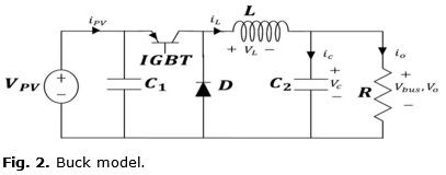
The buck converter circuit used has a capacitor at the connection point with the solar panel, as can be seen in <a href="#fig2">Figure 2</a>, to be able to take V<sub>PV</sub> as a state.</font></p>  	    <p align="center"><a name="fig2"/><img src="/img/revistas/eac/v38n1/f0207117.jpg" width="407" height="160"> 	    <p align="justify"><font face="verdana" size="2">Three states are taken into account in the model, which are: the voltage given by the solar panel V<sub>PV</sub>, the voltage at the output load resistor V<sub>O</sub> and the current flowing through the inductor i<sub>l</sub></font></p>  	    <p align="justify"><font face="verdana" size="2"><img src="/img/revistas/eac/v38n1/i0707117.gif"></font></p>  	    <p align="justify"><font face="verdana" size="2">
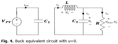
Two models are obtained depending on the state of the IGBT control input u; afterwards, these are combined into a single state space model, which will be used for the identification.
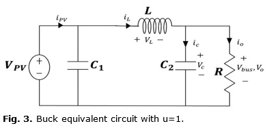
</font></p>  	    ]]></body>
<body><![CDATA[<p align="justify"><font face="verdana" size="2">When the IGBT is in conduction mode (u=1), the equivalent circuit can be seen in <a href="#fig3">Figure 3</a>. The corresponding state space is defined as:</font></p>  	    <p align="justify"><a name="ec13"/><img src="/img/revistas/eac/v38n1/e1307117.gif">  	    <p align="center"><a name="fig3"/><img src="/img/revistas/eac/v38n1/f0307117.jpg" width="391" height="184"> 	    <p align="justify"><font face="verdana" size="2">When the IGBT is in non&#45;conduction mode (u=0), the equivalent circuit can be seen in <a href="#fig4">Figure 4</a>. This way, the state space is defined as:</font></p>  	    <p align="justify"><a name="ec14"/><img src="/img/revistas/eac/v38n1/e1407117.gif">  	     <p align="justify"><font face="verdana" size="2">From the state spaces <a href="#ec13">(13)</a>    and <a href="#ec14">(14)</a>, a new state space model can be obtained:</font></p>  	    <p align="justify"><a name="ec15"/><img src="/img/revistas/eac/v38n1/e1507117.gif">  	    <p align="justify"><font face="verdana" size="2">where,</font></p>  	    <p align="justify"><font face="verdana" size="2"><img src="/img/revistas/eac/v38n1/i0807117.gif"></font></p>  	    <p align="center"><a name="fig4"/><img src="/img/revistas/eac/v38n1/f0407117.jpg" width="412" height="155"> 	    ]]></body>
<body><![CDATA[<p align="justify"><font face="verdana" size="2">The model <a href="#ec15">(15)</a> can also be written as:</font></p>  	    <p align="justify"><a name="ec16"/><img src="/img/revistas/eac/v38n1/e1607117.gif">  	    <p align="justify"><font face="verdana" size="2">Where, </font></p> 	    <p align="justify"><font face="verdana" size="2"><img src="/img/revistas/eac/v38n1/i0907117.gif"></font></p> 	    <p align="justify"><font face="verdana" size="2">In order to obtain a discrete&#45;time model, the Euler discretization method is used:</font></p>  	    <p align="justify"><a name="ec17"/><img src="/img/revistas/eac/v38n1/e1707117.gif">  	    <p align="justify"><font face="verdana" size="2">with,</font></p> 	    <p align="justify"><font face="verdana" size="2"><img src="/img/revistas/eac/v38n1/i1007117.gif"></font></p> 	    <p align="justify"><font face="verdana" size="2"><b>3.2.&#45; IDENTIFICATION</b></font></p>  	     <p align="justify"><font face="verdana" size="2">Based on the structure of <a href="#ec17">(17)</a>,    the RHONN proposed for the DC&#45;DC Buck converter is defined as follows:</font></p>  	    ]]></body>
<body><![CDATA[<p align="justify"><a name="ec18"/><img src="/img/revistas/eac/v38n1/e1807117.gif">  	     <p align="justify"><font face="verdana" size="2">where, S(&#8729;) is a logistic    function, as was seen in the mathematical preliminaries. The second and third    equations in <a href="#ec18">(18)</a> correspond to the internal dynamics of    the system. The second equation describes the dynamics of the voltage at the    load resistor of the buck converter; due to the nature of the converter, this    voltage will always be lower than V<sub>PV</sub>. The third equation represents    the dynamics of the current through the inductor. The weight vectors are updated    online using the extended Kalman filter (EKF), the estimation error is defined    by:</font></p>  	    <p align="justify"><a name="ec19"/><img src="/img/revistas/eac/v38n1/e1907117.gif">  	    <p align="justify"><font face="verdana" size="2">It is worth to note that the states need to be measurable.</font></p>  	    <p align="justify"><font face="verdana" size="2"><b>3.3.&#45; CONTROL DESIGN</b></font></p>  	    <p align="justify"><font face="verdana" size="2">The control is based on the identification described in the previous subsection, its objective is that the voltage at the output of the solar panel reaches the trajectory, x<sub>1</sub><sup>ref</sup>given by the MPPT, and then the tracking error is defined as:</font></p>  	    <p align="justify"><a name="ec20"/><img src="/img/revistas/eac/v38n1/e2007117.gif">  	    <p align="justify"><font face="verdana" size="2">The dynamic error is obtained evaluating <a href="#ec20">(20)</a> at stepk+1, as follows:</font></p>  	    <p align="justify"><a name="ec21"/><img src="/img/revistas/eac/v38n1/e2107117.gif">  	    <p align="justify"><font face="verdana" size="2">The desired dynamic error is e<sub>k+1</sub>= k<sub>1</sub>e<sub>k</sub>,which implies a control law as:</font></p>  	    ]]></body>
<body><![CDATA[<p align="justify"><a name="ec22"/><img src="/img/revistas/eac/v38n1/e2207117.gif">  	    <p align="justify"><font face="verdana" size="2">where, 0&lt; k<sub>1</sub>&#8804;1 is a control design constant to minimize the error asymptotically.</font></p>  	    <p align="justify">&nbsp;</p>  	    <p align="justify"><font face="verdana" size="3"><b>4.&#45;</b> <b>SIMULATION RESULTS</b></font></p>  	    <p align="justify">&nbsp;</p>  	     <p align="justify"><font face="verdana" size="2">In order to test the performance    of the proposed neural controller, a simulation is developed implementing the    DC&#45;DC Buck converter and the solar panel by means of the Simscape Power    Systems <a name="_ftnref2"></a><a href="#_ftn2" title=""><sup>2</sup></a> blocks,    which includes the models of the electrical components, allowing to investigate    to some degree the real&#45;time performance of the proposed design and this    way have a better idea of the necessary considerations for real&#45;time implementation.</font></p>  	    <p align="justify"><font face="verdana" size="2">
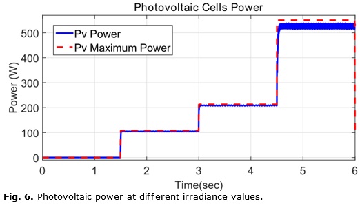
For the realized test, the PV array simulated is the Soltech 1STH&#45;215&#45;P, with parameters described in <a href="#tab1">Table 1</a>. The simulation scheme is shown in <a href=/img/revistas/eac/v38n1/f0507117.jpg">Figure 5</a>, where it can be seen that the temperature in the cells is considered constant at 25 ºC. At the beginning a 0 W/m<sup>2</sup> irradiance is applied, then at 1.5 seconds it is increased to 500 W/m<sup>2</sup>, finally at 3 and 4.5 seconds the irradiance is changed to 1000 W/m<sup>2</sup> and 3000 W/m<sup>2</sup> respectively. At the beginning of the simulation the plant is left in open&#45;loop, having as input a linear swept&#45;frequency cosine signal, this time is used to identify the states. At 0.2 seconds the loop is closed and the controller starts to operate. The objective of the controller is to allow the solar panel to function at the highest efficiency possible, which means producing the maximum amount of power according to its characteristics and environmental conditions at each moment. In <a href="#fig6">Figure 6</a>, the theoretical maximum power level given by <a href="#ec1">(1)</a> for the particular solar panel chosen and applying the previously described irradiance values, is shown in the red dotted line. The blue line represents the power obtained at the output of the solar panel, controlled by the proposed controller as it follows the referenced given by the MPPT algorithm. At the beginning, without solar irradiance, the theoretical maximum power and the actual power obtained are both obviously zero. When irradiance is applied, it can be seen that the actual power quickly converges to the theoretical maximum power with acceptable tracking error. The biggest error is seen at the final irradiance change, this error can be attributed to the dissipation of power from the various components of the converter and the error in the reference given by the MPPT algorithm. As the demand of power increases, the difference between the theoretical maximum power and the reference given by the MPPT algorithm increases as well, reaching an error of up to 7% from the theoretical maximum power. &nbsp;</font></p>  	    
<p align="center"><a name="tab1"/><img src="/img/revistas/eac/v38n1/t0107117.gif" width="456" height="234"> 	    <p align="center"><a name="fig6"/><img src="/img/revistas/eac/v38n1/f0607117.jpg" width="522" height="296"> 	    <p align="justify"><font face="verdana" size="2">In <a href="#fig7">Figure 7</a>, the identification errors are shown. During the first instant the error is quite large because the states of the neural network start in random locations, but the error diminishes almost instantly. After the training or identification time of 0.2 seconds, and while the irradiance remains null, the identification error of the all states is practically zero. When irradiance is first applied at 1.5 seconds, there is a peak of .1V and 0.01A in the error of the first and third states respectively; this doesn't cause a significant problem for tracking the desired output power. It can be seen that the first state, which is the voltage at the output of the solar panel, is the one with the largest estimation error; nevertheless the errors remain within adequate bounds for the entire simulation. Some changes in the amplitude of the estimation error are noticeable every time the irradiance value changes.</font></p>  	    ]]></body>
<body><![CDATA[<p align="justify"><font face="verdana" size="2">In order to compare the proposed neural algorithm with a different controller of the same class, an additional simulation is performed using a discrete sliding mode controller (DSM) based on &#91;19&#93;. Since one of the main advantages of using on&#45;line identification and control is to be able to withstand parametric changes in the model caused by variations in the environment, in this simulation, parametric changes in the DC&#45;DC Buck converter components (capacitors and inductors) are applied. To compare the proposed controller with the DSM controller, tracking error statistics of both are analyzed.</font></p>  	     <p align="justify"><font face="verdana" size="2"><a href=/img/revistas/eac/v38n1/t0207117.gif">Table    2</a>, shows the mean and the standard deviation (SD) of the error with negative    changes in capacitance and inductance values to different percentages, shown    in the left column. The best values for each statistical measure are emphasized    in bold. The least amount of standard deviation in the error is achieved with    the neural controller when there are no parametric</font></p>  	    
<p align="center"><a name="fig7"/><img src="/img/revistas/eac/v38n1/f0707117.jpg" width="507" height="298"> 	     <p align="justify"><font face="verdana" size="2">changes, and the lowest value    for the error mean is achieved with the DSM controller with a 20% change in    the parameter values. It is evident that the error mean is lower when using    the DSM controller but the SD grows as the parametric changes increase, meanwhile    the neural controller mean and SD remain mostly constant. The error in the mean    of the neural controller can be attributed to the always existing identification    errors, but this way it is shown that the same controller can be used for a    completely different converter and very similar results as with the original    will be obtained.</font></p>  	    <p align="justify">&nbsp;</p>  	    <p align="justify"><font face="verdana" size="3"><b>5.&#45;</b> <b>CONCLUSIONS</b></font></p>  	    <p align="justify">&nbsp;</p>  	     <p align="justify"><font face="verdana" size="2">This paper presents a novel application    of the neural network on&#45;line identification using the EKF as in &#91;10&#93;    to achieve a photovoltaic panel MPP reference tracking under varying working    conditions. The MPPT method used was the <i>perturb and observe</i> algorithm,    which is the most common even though it may result in oscillations of the power    output reference if a proper strategy is not adopted. Although the MPPT algorithm    used has a slightly larger error from the theoretical maximum power as the demand    of power increases, by choosing an appropriate step size it was shown that the    theoretical maximum power point was reached with an error of less than 8% under    all irradiance values applied in this work. The on&#45;line method for identification    applied provides robustness against parametric changes in the components, although    it is important to note that the states must be measurable, which in this case    would mean having voltage and current sensors for the DC&#45;DC Buck converter,    which is not considered to be an important impediment. The simulations were    developed using the Simscape Power Systems blocks, which provide component libraries    and analysis tools for modeling and simulating electrical power systems, and    include the different component dynamics and the model of the photovoltaic array,    establishing the basis for a real&#45;time implementation. In the first simulation    presented, irradiance values changed instantly at different points in time and    with the presented controller the solar panel was able to produce the maximum    amount of power according to its particular characteristics. Considering that    in a real application irradiance values would not change instantly, but rather    as a smooth function, the controller is expected to function in a similar manner,    and there would not be abrupt changes in the states. This would be an improvement    that can be applied to the simulation to see how well it responds to ramp changes    and smooth irradiance variations. In the following simulations, the same irradiance    changes were applied and the performance of the proposed controller was validated    compared to a DSM controller while applying different amounts of parametric    change to the DC&#45;DC Buck converter in each simulation. In these simulations    it was shown that the proposed controller has high precision and small convergence    time even when working with a converter that has changed significantly due to    environmental factors, or even with a different converter. It is left as future    work to implement changes in temperature as the irradiance varies, which would    represent more closely the working conditions of a solar panel. This work represents    the basis for the real&#45;time implementation of the proposed controller, which    would greatly improve the performance of solar panels under several conditions,    especially those used in the private sector represented by citizens who invest    in these systems. A different study would need to be realized to be able to    determine the extent of utility of these results for the industrial sector.    The results obtained in this work are important for photovoltaic system users    to be able to obtain the highest efficiency from their solar panels and this    way generate the highest revenue possible, regardless of the climate changes.</font></p>  	    <p align="justify">&nbsp;</p>  	    <p align="justify"><strong><font face="verdana" size="3">REFERENCES</font></strong></p> 	    ]]></body>
<body><![CDATA[<p align="justify">&nbsp;</p> 	    <!-- ref --><p align="justify"><font face="verdana" size="2">1.&nbsp;&nbsp;&nbsp;Hadjab M, Berrah S, Abid H. Neural Network for Modeling Solar Panel. International Journal of Energy. 2012;6(1):9&#45;16.    </font></p>  	    <!-- ref --><p align="justify"><font face="verdana" size="2">2.&nbsp;&nbsp;&nbsp;Syafaruddin KE, Hiyama T. Artificial Neural Network&#45;Polar Coordinated Fuzzy Controller Based Maximum Power Point Tracking Control under Partially Shaded Conditions. IET Renewable Power Generation. 2009;3(2):239&#45;253.    </font></p>  	    <!-- ref --><p align="justify"><font face="verdana" size="2">3.&nbsp;&nbsp;&nbsp;Bastidas&#45;Rodriguez JK, Franco E, Petrone G, Ramos&#45;Paja AC, Spagnuolo G. Maximum Power Point Tracking Architectures for Photovoltaic Systems in Mismatching Conditions: a review. IET Power Electronics. 2014;7(6):1396&#45;1413.    </font></p>  	    <!-- ref --><p align="justify"><font face="verdana" size="2">4.&nbsp;&nbsp;&nbsp;Chatterjee A, Keyhani A. Neural Network Estimation of Microgrid Maximum Solar Power. IEEE Transactions on Smart Grid. 2012;3(4):1860&#45;1866.    </font></p>  	     <!-- ref --><p align="justify"><font face="verdana" size="2">5.&nbsp;&nbsp;&nbsp;Nedumgatt    J, Jayakrishnan K, Umashankar S, Vijavakumar D, Kothari D. Perturb and Observe    MPPT Algorirthm for Solar PV Systems&#45;Modeling and Simulation. In: 2011 Annual    IEEE India Conference, Hyderabad(India); 2011. p.1&#45;6</font><!-- ref --><p align="justify"><font face="verdana" size="2">6.&nbsp;&nbsp;&nbsp;Ahmed AS,    Abdullah BA, Abdelaal WGA. MPPT Algorithms: Performance and Evaluation. In:    2016 11<sup>th</sup> International Conference on Computer Engineering Systems(ICCES),    Cairo (Egypt); 2016. p. 461&#45;467.    </font></p>  	    <!-- ref --><p align="justify"><font face="verdana" size="2">7.&nbsp;&nbsp;&nbsp;Cubas J, Pindado S, De Manuel C. Explicit Expressions for Solar Panel Equivalent Circuit Parameters Based on Analytical Formulation and the Lambert W&#45;function. Energies. 2014;7(7):4098&#45;4115.    </font></p>  	    <!-- ref --><p align="justify"><font face="verdana" size="2">8.&nbsp;&nbsp;&nbsp;Esram T, Chapman PL. Comparison of Photovoltaic Array Maximum Power Point Tracking Techniques. IEEE Transactions on Energy Conversion. 2007;22(2):439&#45;449.    </font></p>  	    <!-- ref --><p align="justify"><font face="verdana" size="2">9.&nbsp;&nbsp;&nbsp;Zhang L, Bai YF. Genetic Algorithm&#45;trained Radial Basis Function Neural Networks for Modelling Photovoltaic Panels. Engineering Applications of Artificial Intelligence. 2005;18(7):833&#45;844.    </font></p>  	     <!-- ref --><p align="justify"><font face="verdana" size="2">10. Sanchez EN, Alanis AY, Loukianov    AG. Discrete&#45;time High Order Neural Control. 1st ed. Warsaw: Springer; 2008.    </font></p>  	    ]]></body>
<body><![CDATA[<!-- ref --><p align="justify"><font face="verdana" size="2">11. Rovithakis GA, Christodoulou MA. Adaptive Control with Recurrent High&#45;order Neural Networks/Theory and Industrial Applications. 1st ed. London: Springer; 2000.    </font></p>  	    <!-- ref --><p align="justify"><font face="verdana" size="2">12. Hailong R, Jidong LV, Cuiyun P, Ling Z, Zhenghua M, Yang C, et al. Dynamic Regulation of the Weights of Request Based on the Kalman Filter and an Artificial Neural Network. IEEE Sensors journal. 2016;16(23):8597&#45;8607.    </font></p>  	     <!-- ref --><p align="justify"><font face="verdana" size="2">13. Brown RG, Hwang PYC. Introduction    to Random Signals and Applied Kalman Filtering with MATLAB Exercises. 4th ed.    Massachusetts: John Wiley &amp; Sons, Inc; 2012.    </font></p>  	     <!-- ref --><p align="justify"><font face="verdana" size="2">14. Bouheraoua M, Wang J, Atallah    K. Rotor Position Estimation of a Pseudo Direct Drive PM Machine Using Extended    Kalman Filter. IEEE Transactions on Industry Applications. 2017;53(2):1088&#45;1095.    </font></p>  	     <!-- ref --><p align="justify"><font face="verdana" size="2">15. Pajchrowski T, Janiszewski    D. Control of Multi&#45;mass System by On&#45;line Trained Neural Network Based    on Kalman Filter. In: 2015 17th European Conference on Power Electronics and    Applications(EPE'15 ECCE&#45;Europe), Geneva(Switzerland); 2015. p.1&#45;10.    </font></p>  	     ]]></body>
<body><![CDATA[<!-- ref --><p align="justify"><font face="verdana" size="2">16. Rajesh MV, Archana R, Unnikrishnan    A, Gopikakaumari R. Comparative Study on EKF Training Algorithm with EM and    MLE for ANN modeling of nonlinear systems. In: 29th Chinese Control Conference,    Beijing(China); 2010. p.1407&#45;1413.    </font></p>  	     <!-- ref --><p align="justify"><font face="verdana" size="2">17. Alanis AY, Sanchez EN, Loukianov    AG. Discrete&#45;time Backstepping Induction Motor Control Using a Sensorless    Recurrent Neural Observer. In: 46th IEEE Conference on Decision and Control,    Louisiana(USA); 2007. p.6112&#45;6117.    </font></p>  	    <!-- ref --><p align="justify"><font face="verdana" size="2">18. Shenglong Y, Kianoush E, Tyrone F, Herber HC, Kit PW. State Estimation of Doubly Fed Induction Generator Wind Turbine in Complex Power Systems. IEEE Transactions on Power Systems. 2016;31(6):4935&#45;4944.    </font></p>  	     <!-- ref --><p align="justify"><font face="verdana" size="2">19. Khiari B, Sellami A, Andoulsi    R, M'Hiri R, Ksouri M. Discrete Control by Sliding Mode of a Photovoltaic System.    In: First International Symposiumon Control, Communications and Signal Processing,    Hammamet(Tunisia); 2004. p.469&#45;474.    </font></p>      <p align="justify">&nbsp;</p>     <p align="justify">&nbsp;</p>     ]]></body>
<body><![CDATA[<p align="justify"><font face="verdana" size="2">Received: 18 de septiembre del    2016&nbsp;&nbsp;&nbsp;&nbsp;&nbsp;&nbsp;    <br>   Approved: 26 de enero del 2017</font></p>     <p align="justify">&nbsp;</p>     <p align="justify">&nbsp;</p>  	    <p align="justify"><font face="verdana" size="2"><em>Mart&iacute;n de Jes&uacute;s Loza&#45;L&oacute;pez</em>, Centro de Investigaci&oacute;n y Estudios Avanzados del Instituto Polit&eacute;cnico Nacional, Jalisco, Mexico. E-mail: <a href="mailto:mdloza@gdl.cinvestav.mx">mdloza@gdl.cinvestav.mx</a></font></p>  	    <p align="justify">&nbsp;</p> 	    <p align="justify">&nbsp;</p> 	 	    <p align="justify"><font face="verdana" size="2"><a name="_ftn1"></a><a href="#_ftnref1" title=""><sup>1</sup></a> Simulink/Simscape Power Systems are trademarks of The MathWorks,Inc.&nbsp;&nbsp;&nbsp;&nbsp;&nbsp;&nbsp;&nbsp;&nbsp;&nbsp;&nbsp;&nbsp;&nbsp;&nbsp;&nbsp;&nbsp;&nbsp;&nbsp;&nbsp;&nbsp;&nbsp;&nbsp;&nbsp;&nbsp;&nbsp;&nbsp;&nbsp;&nbsp;&nbsp;&nbsp;&nbsp;&nbsp;&nbsp;&nbsp;&nbsp;&nbsp;&nbsp;&nbsp;&nbsp;&nbsp;&nbsp;&nbsp;&nbsp;&nbsp;&nbsp;&nbsp;&nbsp;&nbsp;&nbsp;&nbsp;&nbsp;&nbsp;&nbsp;&nbsp;&nbsp;&nbsp;&nbsp;&nbsp;&nbsp;&nbsp;&nbsp;&nbsp;&nbsp;&nbsp;&nbsp;&nbsp;&nbsp;&nbsp;&nbsp;</font></p>  	    <p align="justify"><font face="verdana" size="2"><a name="_ftn2"></a><a href="#_ftnref2" title=""><sup>2</sup></a> Simscape Power Systems is a trademark of The MathWorks, Inc.</font></p>      ]]></body><back>
<ref-list>
<ref id="B1">
<label>1</label><nlm-citation citation-type="journal">
<person-group person-group-type="author">
<name>
<surname><![CDATA[Hadjab]]></surname>
<given-names><![CDATA[M]]></given-names>
</name>
<name>
<surname><![CDATA[Berrah]]></surname>
<given-names><![CDATA[S]]></given-names>
</name>
<name>
<surname><![CDATA[Abid]]></surname>
<given-names><![CDATA[H]]></given-names>
</name>
</person-group>
<article-title xml:lang="en"><![CDATA[Neural Network for Modeling Solar Panel]]></article-title>
<source><![CDATA[International Journal of Energy]]></source>
<year>2012</year>
<volume>6</volume>
<numero>1</numero>
<issue>1</issue>
<page-range>9-16</page-range></nlm-citation>
</ref>
<ref id="B2">
<label>2</label><nlm-citation citation-type="journal">
<person-group person-group-type="author">
<name>
<surname><![CDATA[Syafaruddin]]></surname>
<given-names><![CDATA[KE]]></given-names>
</name>
<name>
<surname><![CDATA[Hiyama]]></surname>
<given-names><![CDATA[T]]></given-names>
</name>
</person-group>
<article-title xml:lang="en"><![CDATA[Artificial Neural Network-Polar Coordinated Fuzzy Controller Based Maximum Power Point Tracking Control under Partially Shaded Conditions]]></article-title>
<source><![CDATA[IET Renewable Power Generation]]></source>
<year>2009</year>
<volume>3</volume>
<numero>2</numero>
<issue>2</issue>
<page-range>239-253</page-range></nlm-citation>
</ref>
<ref id="B3">
<label>3</label><nlm-citation citation-type="journal">
<person-group person-group-type="author">
<name>
<surname><![CDATA[Bastidas-Rodriguez]]></surname>
<given-names><![CDATA[JK]]></given-names>
</name>
<name>
<surname><![CDATA[Franco]]></surname>
<given-names><![CDATA[E]]></given-names>
</name>
<name>
<surname><![CDATA[Petrone]]></surname>
<given-names><![CDATA[G]]></given-names>
</name>
<name>
<surname><![CDATA[Ramos-Paja]]></surname>
<given-names><![CDATA[AC]]></given-names>
</name>
<name>
<surname><![CDATA[Spagnuolo]]></surname>
<given-names><![CDATA[G]]></given-names>
</name>
</person-group>
<article-title xml:lang="en"><![CDATA[Maximum Power Point Tracking Architectures for Photovoltaic Systems in Mismatching Conditions: a review]]></article-title>
<source><![CDATA[IET Power Electronics]]></source>
<year>2014</year>
<volume>7</volume>
<numero>6</numero>
<issue>6</issue>
<page-range>1396-1413</page-range></nlm-citation>
</ref>
<ref id="B4">
<label>4</label><nlm-citation citation-type="journal">
<person-group person-group-type="author">
<name>
<surname><![CDATA[Chatterjee]]></surname>
<given-names><![CDATA[A]]></given-names>
</name>
<name>
<surname><![CDATA[Keyhani]]></surname>
<given-names><![CDATA[A]]></given-names>
</name>
</person-group>
<article-title xml:lang="en"><![CDATA[Neural Network Estimation of Microgrid Maximum Solar Power]]></article-title>
<source><![CDATA[IEEE Transactions on Smart Grid]]></source>
<year>2012</year>
<volume>3</volume>
<numero>4</numero>
<issue>4</issue>
<page-range>1860-1866</page-range></nlm-citation>
</ref>
<ref id="B5">
<label>5</label><nlm-citation citation-type="">
<person-group person-group-type="author">
<name>
<surname><![CDATA[Nedumgatt]]></surname>
<given-names><![CDATA[J]]></given-names>
</name>
<name>
<surname><![CDATA[Jayakrishnan]]></surname>
<given-names><![CDATA[K]]></given-names>
</name>
<name>
<surname><![CDATA[Umashankar]]></surname>
<given-names><![CDATA[S]]></given-names>
</name>
<name>
<surname><![CDATA[Vijavakumar]]></surname>
<given-names><![CDATA[D]]></given-names>
</name>
<name>
<surname><![CDATA[Kothari]]></surname>
<given-names><![CDATA[D]]></given-names>
</name>
</person-group>
<article-title xml:lang="en"><![CDATA[Perturb and Observe MPPT Algorirthm for Solar PV Systems-Modeling and Simulation]]></article-title>
<source><![CDATA[2011 Annual IEEE India Conference,]]></source>
<year>2011</year>
<page-range>1-6</page-range><publisher-loc><![CDATA[Hyderabad ]]></publisher-loc>
</nlm-citation>
</ref>
<ref id="B6">
<label>6</label><nlm-citation citation-type="">
<person-group person-group-type="author">
<name>
<surname><![CDATA[Ahmed]]></surname>
<given-names><![CDATA[AS]]></given-names>
</name>
<name>
<surname><![CDATA[Abdullah]]></surname>
<given-names><![CDATA[BA]]></given-names>
</name>
<name>
<surname><![CDATA[Abdelaal]]></surname>
<given-names><![CDATA[WGA]]></given-names>
</name>
</person-group>
<article-title xml:lang="en"><![CDATA[MPPT Algorithms: Performance and Evaluation]]></article-title>
<source><![CDATA[2016 11th International Conference on Computer Engineering Systems(ICCES),]]></source>
<year>2016</year>
<page-range>461-467</page-range><publisher-loc><![CDATA[Cairo ]]></publisher-loc>
</nlm-citation>
</ref>
<ref id="B7">
<label>7</label><nlm-citation citation-type="journal">
<person-group person-group-type="author">
<name>
<surname><![CDATA[Cubas]]></surname>
<given-names><![CDATA[J]]></given-names>
</name>
<name>
<surname><![CDATA[Pindado]]></surname>
<given-names><![CDATA[S]]></given-names>
</name>
<name>
<surname><![CDATA[De Manuel]]></surname>
<given-names><![CDATA[C]]></given-names>
</name>
</person-group>
<article-title xml:lang="en"><![CDATA[Explicit Expressions for Solar Panel Equivalent Circuit Parameters Based on Analytical Formulation and the Lambert W-function]]></article-title>
<source><![CDATA[Energies]]></source>
<year>2014</year>
<volume>7</volume>
<numero>7</numero>
<issue>7</issue>
<page-range>4098-4115</page-range></nlm-citation>
</ref>
<ref id="B8">
<label>8</label><nlm-citation citation-type="journal">
<person-group person-group-type="author">
<name>
<surname><![CDATA[Esram]]></surname>
<given-names><![CDATA[T]]></given-names>
</name>
<name>
<surname><![CDATA[Chapman]]></surname>
<given-names><![CDATA[PL]]></given-names>
</name>
</person-group>
<article-title xml:lang="en"><![CDATA[Comparison of Photovoltaic Array Maximum Power Point Tracking Techniques]]></article-title>
<source><![CDATA[IEEE Transactions on Energy Conversion]]></source>
<year>2007</year>
<volume>22</volume>
<numero>2</numero>
<issue>2</issue>
<page-range>439-449</page-range></nlm-citation>
</ref>
<ref id="B9">
<label>9</label><nlm-citation citation-type="journal">
<person-group person-group-type="author">
<name>
<surname><![CDATA[Zhang]]></surname>
<given-names><![CDATA[L]]></given-names>
</name>
<name>
<surname><![CDATA[Bai]]></surname>
<given-names><![CDATA[YF]]></given-names>
</name>
</person-group>
<article-title xml:lang="en"><![CDATA[Genetic Algorithm-trained Radial Basis Function Neural Networks for Modelling Photovoltaic Panels]]></article-title>
<source><![CDATA[Engineering Applications of Artificial Intelligence]]></source>
<year>2005</year>
<volume>18</volume>
<numero>7</numero>
<issue>7</issue>
<page-range>833-844</page-range></nlm-citation>
</ref>
<ref id="B10">
<label>10</label><nlm-citation citation-type="book">
<person-group person-group-type="author">
<name>
<surname><![CDATA[Sanchez]]></surname>
<given-names><![CDATA[EN]]></given-names>
</name>
<name>
<surname><![CDATA[Alanis]]></surname>
<given-names><![CDATA[AY]]></given-names>
</name>
<name>
<surname><![CDATA[Loukianov]]></surname>
<given-names><![CDATA[AG]]></given-names>
</name>
</person-group>
<source><![CDATA[Discrete-time High Order Neural Control]]></source>
<year>2008</year>
<edition>1</edition>
<publisher-loc><![CDATA[Warsaw ]]></publisher-loc>
<publisher-name><![CDATA[Springer]]></publisher-name>
</nlm-citation>
</ref>
<ref id="B11">
<label>11</label><nlm-citation citation-type="book">
<person-group person-group-type="author">
<name>
<surname><![CDATA[Rovithakis]]></surname>
<given-names><![CDATA[GA]]></given-names>
</name>
<name>
<surname><![CDATA[Christodoulou]]></surname>
<given-names><![CDATA[MA]]></given-names>
</name>
</person-group>
<source><![CDATA[Adaptive Control with Recurrent High-order Neural Networks/Theory and Industrial Applications]]></source>
<year>2000</year>
<edition>1</edition>
<publisher-loc><![CDATA[London ]]></publisher-loc>
<publisher-name><![CDATA[Springer]]></publisher-name>
</nlm-citation>
</ref>
<ref id="B12">
<label>12</label><nlm-citation citation-type="journal">
<person-group person-group-type="author">
<name>
<surname><![CDATA[Hailong]]></surname>
<given-names><![CDATA[R]]></given-names>
</name>
<name>
<surname><![CDATA[Jidong]]></surname>
<given-names><![CDATA[LV]]></given-names>
</name>
<name>
<surname><![CDATA[Cuiyun]]></surname>
<given-names><![CDATA[P]]></given-names>
</name>
<name>
<surname><![CDATA[Ling]]></surname>
<given-names><![CDATA[Z]]></given-names>
</name>
<name>
<surname><![CDATA[Zhenghua]]></surname>
<given-names><![CDATA[M]]></given-names>
</name>
<name>
<surname><![CDATA[Yang]]></surname>
<given-names><![CDATA[C]]></given-names>
</name>
</person-group>
<article-title xml:lang="en"><![CDATA[Dynamic Regulation of the Weights of Request Based on the Kalman Filter and an Artificial Neural Network]]></article-title>
<source><![CDATA[IEEE Sensors journal]]></source>
<year>2016</year>
<volume>16</volume>
<numero>23</numero>
<issue>23</issue>
<page-range>8597-8607</page-range></nlm-citation>
</ref>
<ref id="B13">
<label>13</label><nlm-citation citation-type="book">
<person-group person-group-type="author">
<name>
<surname><![CDATA[Brown]]></surname>
<given-names><![CDATA[RG]]></given-names>
</name>
<name>
<surname><![CDATA[Hwang]]></surname>
<given-names><![CDATA[PYC]]></given-names>
</name>
</person-group>
<source><![CDATA[Introduction to Random Signals and Applied Kalman Filtering with MATLAB Exercises]]></source>
<year>2012</year>
<edition>4</edition>
<publisher-loc><![CDATA[Massachusetts ]]></publisher-loc>
<publisher-name><![CDATA[John Wiley & Sons, Inc]]></publisher-name>
</nlm-citation>
</ref>
<ref id="B14">
<label>14</label><nlm-citation citation-type="journal">
<person-group person-group-type="author">
<name>
<surname><![CDATA[Bouheraoua]]></surname>
<given-names><![CDATA[M]]></given-names>
</name>
<name>
<surname><![CDATA[Wang]]></surname>
<given-names><![CDATA[J]]></given-names>
</name>
<name>
<surname><![CDATA[Atallah]]></surname>
<given-names><![CDATA[K]]></given-names>
</name>
</person-group>
<article-title xml:lang="en"><![CDATA[Rotor Position Estimation of a Pseudo Direct Drive PM Machine Using Extended Kalman Filter]]></article-title>
<source><![CDATA[IEEE Transactions on Industry Applications]]></source>
<year>2017</year>
<volume>53</volume>
<numero>2</numero>
<issue>2</issue>
<page-range>1088-1095</page-range></nlm-citation>
</ref>
<ref id="B15">
<label>15</label><nlm-citation citation-type="">
<person-group person-group-type="author">
<name>
<surname><![CDATA[Pajchrowski]]></surname>
<given-names><![CDATA[T]]></given-names>
</name>
<name>
<surname><![CDATA[Janiszewski]]></surname>
<given-names><![CDATA[D]]></given-names>
</name>
</person-group>
<article-title xml:lang="en"><![CDATA[Control of Multi-mass System by On-line Trained Neural Network Based on Kalman Filter]]></article-title>
<source><![CDATA[2015 17th European Conference on Power Electronics and Applications(EPE'15 ECCE-Europe),]]></source>
<year>2015</year>
<page-range>1-10</page-range><publisher-loc><![CDATA[Geneva ]]></publisher-loc>
</nlm-citation>
</ref>
<ref id="B16">
<label>16</label><nlm-citation citation-type="">
<person-group person-group-type="author">
<name>
<surname><![CDATA[Rajesh]]></surname>
<given-names><![CDATA[MV]]></given-names>
</name>
<name>
<surname><![CDATA[Archana]]></surname>
<given-names><![CDATA[R]]></given-names>
</name>
<name>
<surname><![CDATA[Unnikrishnan]]></surname>
<given-names><![CDATA[A]]></given-names>
</name>
<name>
<surname><![CDATA[Gopikakaumari]]></surname>
<given-names><![CDATA[R]]></given-names>
</name>
</person-group>
<article-title xml:lang="en"><![CDATA[Comparative Study on EKF Training Algorithm with EM and MLE for ANN modeling of nonlinear systems]]></article-title>
<source><![CDATA[29th Chinese Control Conference,]]></source>
<year>2010</year>
<page-range>1407-1413</page-range><publisher-loc><![CDATA[Beijing ]]></publisher-loc>
</nlm-citation>
</ref>
<ref id="B17">
<label>17</label><nlm-citation citation-type="">
<person-group person-group-type="author">
<name>
<surname><![CDATA[Alanis]]></surname>
<given-names><![CDATA[AY]]></given-names>
</name>
<name>
<surname><![CDATA[Sanchez]]></surname>
<given-names><![CDATA[EN]]></given-names>
</name>
<name>
<surname><![CDATA[Loukianov]]></surname>
<given-names><![CDATA[AG]]></given-names>
</name>
</person-group>
<article-title xml:lang="en"><![CDATA[Discrete-time Backstepping Induction Motor Control Using a Sensorless Recurrent Neural Observer]]></article-title>
<source><![CDATA[46th IEEE Conference on Decision and Control,]]></source>
<year>2007</year>
<page-range>6112-6117</page-range><publisher-loc><![CDATA[Louisiana ]]></publisher-loc>
</nlm-citation>
</ref>
<ref id="B18">
<label>18</label><nlm-citation citation-type="journal">
<person-group person-group-type="author">
<name>
<surname><![CDATA[Shenglong]]></surname>
<given-names><![CDATA[Y]]></given-names>
</name>
<name>
<surname><![CDATA[Kianoush]]></surname>
<given-names><![CDATA[E]]></given-names>
</name>
<name>
<surname><![CDATA[Tyrone]]></surname>
<given-names><![CDATA[F]]></given-names>
</name>
<name>
<surname><![CDATA[Herber]]></surname>
<given-names><![CDATA[HC]]></given-names>
</name>
<name>
<surname><![CDATA[Kit]]></surname>
<given-names><![CDATA[PW]]></given-names>
</name>
</person-group>
<article-title xml:lang="en"><![CDATA[State Estimation of Doubly Fed Induction Generator Wind Turbine in Complex Power Systems]]></article-title>
<source><![CDATA[IEEE Transactions on Power Systems]]></source>
<year>2016</year>
<volume>31</volume>
<numero>6</numero>
<issue>6</issue>
<page-range>4935-4944</page-range></nlm-citation>
</ref>
<ref id="B19">
<label>19</label><nlm-citation citation-type="">
<person-group person-group-type="author">
<name>
<surname><![CDATA[Khiari]]></surname>
<given-names><![CDATA[B]]></given-names>
</name>
<name>
<surname><![CDATA[Sellami]]></surname>
<given-names><![CDATA[A]]></given-names>
</name>
<name>
<surname><![CDATA[Andoulsi]]></surname>
<given-names><![CDATA[R]]></given-names>
</name>
<name>
<surname><![CDATA[M'Hiri]]></surname>
<given-names><![CDATA[R]]></given-names>
</name>
<name>
<surname><![CDATA[Ksouri]]></surname>
<given-names><![CDATA[M]]></given-names>
</name>
</person-group>
<article-title xml:lang="en"><![CDATA[Discrete Control by Sliding Mode of a Photovoltaic System]]></article-title>
<source><![CDATA[First International Symposiumon Control, Communications and Signal Processing,]]></source>
<year>2004</year>
<page-range>469-474</page-range><publisher-loc><![CDATA[Hammamet ]]></publisher-loc>
</nlm-citation>
</ref>
</ref-list>
</back>
</article>
