<?xml version="1.0" encoding="ISO-8859-1"?><article xmlns:mml="http://www.w3.org/1998/Math/MathML" xmlns:xlink="http://www.w3.org/1999/xlink" xmlns:xsi="http://www.w3.org/2001/XMLSchema-instance">
<front>
<journal-meta>
<journal-id>2079-3480</journal-id>
<journal-title><![CDATA[Cuban Journal of Agricultural Science]]></journal-title>
<abbrev-journal-title><![CDATA[Cuban J. Agric. Sci.]]></abbrev-journal-title>
<issn>2079-3480</issn>
<publisher>
<publisher-name><![CDATA[Editorial del Instituto de Ciencia Animal]]></publisher-name>
</publisher>
</journal-meta>
<article-meta>
<article-id>S2079-34802016000100004</article-id>
<title-group>
<article-title xml:lang="en"><![CDATA[The bootstrap: a 35 years old young very useful for analyzing biological data]]></article-title>
<article-title xml:lang="es"><![CDATA[El bootstrap: un joven de 35 años muy útil para analizar datos biológicos]]></article-title>
</title-group>
<contrib-group>
<contrib contrib-type="author">
<name>
<surname><![CDATA[Navarro Alberto]]></surname>
<given-names><![CDATA[J. A]]></given-names>
</name>
<xref ref-type="aff" rid="A01"/>
</contrib>
</contrib-group>
<aff id="A01">
<institution><![CDATA[,Universidad Autónoma de Yucatán Departamento de Ecología Tropical Campus de Ciencias Biológicas y Agropecuarias ]]></institution>
<addr-line><![CDATA[Mérida Yucatán]]></addr-line>
<country>México</country>
</aff>
<pub-date pub-type="pub">
<day>00</day>
<month>03</month>
<year>2016</year>
</pub-date>
<pub-date pub-type="epub">
<day>00</day>
<month>03</month>
<year>2016</year>
</pub-date>
<volume>50</volume>
<numero>1</numero>
<fpage>11</fpage>
<lpage>23</lpage>
<copyright-statement/>
<copyright-year/>
<self-uri xlink:href="http://scielo.sld.cu/scielo.php?script=sci_arttext&amp;pid=S2079-34802016000100004&amp;lng=en&amp;nrm=iso"></self-uri><self-uri xlink:href="http://scielo.sld.cu/scielo.php?script=sci_abstract&amp;pid=S2079-34802016000100004&amp;lng=en&amp;nrm=iso"></self-uri><self-uri xlink:href="http://scielo.sld.cu/scielo.php?script=sci_pdf&amp;pid=S2079-34802016000100004&amp;lng=en&amp;nrm=iso"></self-uri><abstract abstract-type="short" xml:lang="en"><p><![CDATA[In diverse scientific discussion forums and in specialized journals the word “bootstrap” has been mentioned or read. Will it be that for analyzing our data we must use boots with straps for its use as support points for jumping? (How odd…but this is the word for word translation!). In this paper the significance and development of the bootstrap is reviewed as rigorous statistical calculation method for data analysis. The diverse algorithms associated with the estimation by bootstrap intervals are shown and its application with the problem relative to mean estimation is explained. Finally mention is made of the implications and limitations of this method, as well as of the great usefulness it has in biological and agricultural sciences which have adopted it as analysis tool since its invention by Bradley Efron (U. of Stanford) since more than 35 years ago]]></p></abstract>
<abstract abstract-type="short" xml:lang="es"><p><![CDATA[En diversos foros de discusión de científicos, en revistas especializadas hemos oído mencionar o leído la palabra “bootstrap”. ¿Será que para analizar nuestros datos debemos usar botas con cintillos y usar éstos como puntos de apoyo para saltar? (¡Que cosa más rara... pero esta es la traducción literal de la palabra!). En este trabajo revisaremos el significado y desarrollo del bootstrap como método estadístico de cómputo intensivo para el análisis de datos. Se mostrarán los diversos algoritmos asociados con la estimación por intervalos bootstrap y se ilustrará su aplicación con el problema relativo a la estimación de la mediana. Finalmente, se hará mención de los alcances y limitaciones de este método, así como la gran utilidad que tiene dentro de las ciencias biológicas y agropecuarias, que las han adoptado como herramienta de análisis desde su invención por Bradley Efron (U. de Stanford) hace más de 35 años]]></p></abstract>
<kwd-group>
<kwd lng="en"><![CDATA[Bootstrap]]></kwd>
<kwd lng="en"><![CDATA[interval of confidence]]></kwd>
<kwd lng="en"><![CDATA[biological data]]></kwd>
<kwd lng="en"><![CDATA[median]]></kwd>
<kwd lng="es"><![CDATA[Bootstrap]]></kwd>
<kwd lng="es"><![CDATA[intervalos de confianza]]></kwd>
<kwd lng="es"><![CDATA[datos biológicos]]></kwd>
<kwd lng="es"><![CDATA[mediana]]></kwd>
</kwd-group>
</article-meta>
</front><body><![CDATA[ <p align="right"><strong>Cuban Journal  of Agricultural Science, 50(1): 11-23, 2016, ISSN: 2079-3480</strong></p>     <p align="right">&nbsp;</p>     <p align="right"><font size="2" face="Verdana, Arial, Helvetica, sans-serif"><b>ORIGINAL ARTICLE</b></font></p>     <p align="justify">&nbsp;</p>     <p align="justify"><font size="4" face="Verdana, Arial, Helvetica, sans-serif"><b>The bootstrap: a 35 years old young very useful for analyzing  biological data</b></font></p>     <p align="justify">&nbsp;</p>     <p align="justify"><font size="3" face="Verdana, Arial, Helvetica, sans-serif"><b>El bootstrap: un joven de 35 años muy útil para analizar datos biológicos</b></font></p>     <p align="justify">&nbsp;</p>     <p align="justify">&nbsp;</p>     <p align="justify"><font size="2" face="Verdana, Arial, Helvetica, sans-serif"><b>J. A. Navarro Alberto,</b><sup><b>I</b></sup></font></p>     ]]></body>
<body><![CDATA[<p align="justify"><font size="2" face="Verdana, Arial, Helvetica, sans-serif"><b> </b></font><font size="2" face="Verdana, Arial, Helvetica, sans-serif"><sup>I</sup>Departamento de Ecología Tropical Campus de Ciencias Biológicas y Agropecuarias Universidad Autónoma de Yucatán Km 15.5 Carretera Mérida-Xmatkuil. CP 97315. Mérida, Yucatán, México. </font></p>     <p align="justify">&nbsp;</p>     <p align="justify">&nbsp;</p> <hr align="JUSTIFY">     <p align="justify"><font size="2" face="Verdana, Arial, Helvetica, sans-serif"><b>ABSTRACT</b></font></p>     <p align="justify"><font size="2" face="Verdana, Arial, Helvetica, sans-serif"><span style=" letter-spacing:.2pt; font-family:'Verdana','sans-serif'; font-size:10.0pt; ">In diverse scientific discussion forums and in specialized journals the  word &ldquo;bootstrap&rdquo; has been mentioned or read. Will it be that for analyzing our  data we must use boots with straps for its use as support points for jumping?  (How odd&hellip;but this is the word for word translation!).&nbsp; In this paper the significance and  development of the bootstrap is reviewed as rigorous statistical calculation  method for data analysis. The diverse algorithms associated with the estimation  by bootstrap intervals are shown and its application with the problem relative  to mean estimation is explained. Finally mention is made of the implications  and limitations of this method, as well as of the great usefulness it has in  biological and agricultural sciences which have adopted it as analysis tool  since its invention by Bradley Efron (U. of Stanford) since more than 35 years  ago</span>.</font></p>     <p align="justify"><font size="2" face="Verdana, Arial, Helvetica, sans-serif"><b>Key words:</b> Bootstrap, interval of confidence, biological data,  median.</font></p> <hr align="JUSTIFY">     <p align="justify"><font size="2" face="Verdana, Arial, Helvetica, sans-serif"><b>RESUMEN</b></font></p>     <p align="justify"><font size="2" face="Verdana, Arial, Helvetica, sans-serif"><span style=" letter-spacing:-.1pt; font-family:'Verdana','sans-serif'; font-size:10.0pt; ">En diversos foros de discusi&oacute;n de cient&iacute;ficos, en  revistas especializadas hemos o&iacute;do mencionar o le&iacute;do la palabra &ldquo;bootstrap&rdquo;.  &iquest;Ser&aacute; que para analizar nuestros datos debemos usar botas con cintillos y usar  &eacute;stos como puntos de apoyo para saltar? (&iexcl;Que cosa m&aacute;s rara... pero esta es la  traducci&oacute;n literal de la palabra!). En este trabajo revisaremos el significado  y desarrollo del bootstrap como m&eacute;todo estad&iacute;stico de c&oacute;mputo intensivo para el  an&aacute;lisis de datos.&nbsp; Se mostrar&aacute;n los  diversos algoritmos asociados con la estimaci&oacute;n por intervalos bootstrap y se  ilustrar&aacute; su aplicaci&oacute;n con el problema relativo a la estimaci&oacute;n de la mediana.  Finalmente, se har&aacute; menci&oacute;n de los alcances y limitaciones de este m&eacute;todo, as&iacute;  como la gran utilidad que tiene dentro de las ciencias biol&oacute;gicas y  agropecuarias, que las han adoptado como herramienta de an&aacute;lisis desde su  invenci&oacute;n por Bradley Efron (U. de Stanford) hace m&aacute;s de 35 a&ntilde;os</span>.</font></p>     <p align="justify"><font size="2" face="Verdana, Arial, Helvetica, sans-serif"><b>Palabras    clave:</b>    Bootstrap, intervalos de confianza, datos biológicos, mediana.</font></p> <hr align="JUSTIFY">     <p align="justify">&nbsp;</p>     ]]></body>
<body><![CDATA[<p align="justify">&nbsp;</p>     <p align="justify"><font size="2" face="Verdana, Arial, Helvetica, sans-serif"><b><font size="3">INTRODUCTION</font></b></font></p>       <p align="justify" class="Cuerpodetexto" style="text-indent:0in;"><span style=" letter-spacing:.2pt; font-family:'Verdana','sans-serif'; font-size:10.0pt; ">In statistics it is customary to discuss about means and  errors (standard) of variables in continuous scale: weights of seven months old  steers, daily milk yield in dairy cows, etc. The strategy for the analysis of  these variables for statistical inference is assuming that there is only  statistical variation and that having a sufficient number of measurements is  enough so as to calculate the mean and the standard error of the mean, knowing  that the standard error decreases as the number of measurements increases. The  artillery of statistical methods in these cases is vast and it is commanded by one  of the most important theorems of Statistics: the Theorem of Central Limit: &ldquo;If  random size samples are taken n, <em>y<sub>1</sub>, y<sub>2</sub>&hellip;y<sub>n</sub></em> of a population with finite mean &micro; and variance &sigma;</span><sup><span style=" letter-spacing:-.1pt; font-family:'Verdana','sans-serif'; font-size:10.0pt; ">2</span></sup><span style="font-family:'Verdana','sans-serif'; font-size:10.0pt; ">, then  for an n sufficiently large, the sampling mean distribution (sampling means)  can be approximated with a function of normal density with mean <em>&micro;</em></span><em><sub><span style=" letter-spacing:.2pt; font-family:'Calibri','sans-serif'; font-size:10.0pt; ">&#563;</span></sub><span style="font-family:'Verdana','sans-serif'; font-size:10.0pt; ">=&micro; </span></em><span style="font-family:'Verdana','sans-serif'; font-size:10.0pt; ">&nbsp;and standard deviation (standard error) <em>&sigma;</em></span><em><sub><span style="font-family:'Calibri','sans-serif'; font-size:10.0pt; ">&#563;</span></sub><span style="font-family:'Verdana','sans-serif'; font-size:10.0pt; ">=&sigma;/&radic;n</span></em><span style="font-family:'Verdana','sans-serif'; font-size:10.0pt; ">. The error that will be committed due to the  approximation of the distribution of the sampling means to the normal will  decrease as n increases. For example, in <a href="/img/revistas/cjas/v50n1/f0104116.gif">figure 1</a>, the sampling distributions  generated on selecting the samples of normal random variables or uniform are  approximately normal even for n as small as 10 (<a href="/img/revistas/cjas/v50n1/f0104116.gif">figures&nbsp; A1, B1</a>). On the other hand, for biased  distributions such as square ji the mean sampling distribution is not normal  for n = 10 (<a href="/img/revistas/cjas/v50n1/f0104116.gif">figure    C1</a>), and only for n values as large as 100 is that this distribution is  practically normal (<a href="/img/revistas/cjas/v50n1/f0104116.gif">figure C2</a>).</span></p>       
<p align="justify" class="Cuerpodetexto" style="text-indent:0in;"><span style="font-family:'Verdana','sans-serif'; font-size:10.0pt; ">In many cases, our variables of interest have unknown  distribution and thus, it is not possible to know how large the sample must be  in order to apply the result of the Theorem of Central Limit.&nbsp; If we rely on the results (asymptotic) of the  Theorem of Central Limit these could not satisfy the level of accuracy with a  relatively small sample. If the suppositions on the population are incorrect,  then the sampling distribution can be quite inaccurate. In addition, it can be  very difficult to deduce mathematically the sampling distribution of the  statistical of interest. All these questions can be latent since with only one  sample of particular size it seems to be impossible establishing which the  sampling distribution is. The idea of the bootstrap focus on this situation:  only one data set is available by hand of a certain size and questions if it is  possible determining the sampling distribution of its data without using the  Theorem of Central Limit.&nbsp; Bootstrapping  is a general approach of statistical inference based on these ideas of creating  the sampling distribution for a statistics through re-sampling of data close at  hand.</span></p>       <p align="justify"><span style=" font-family:'Verdana','sans-serif'; font-size:10.0pt; ">The formalization of the  bootstrap method is owed to Bradley Efron (Efron 1979 and Efron and Tibshirani  1993) who took ideas from various precursor statistical procedures: the random  sampling of finite populations, the estimation of variances from various  samplings, stratified semi-samplings and inference methods of intensive  calculation, specially Monte Carlo and the jackknife.&nbsp; Efron describes in the above mentioned paper  the difficult decision for choosing the name of the method, motivated by the  audacity of Tukey (1958) for naming in a special way his methods (jackknife,  stem and leaf diagram, box and mustache graphic). Tukey proposed the jackknife  by analogy with those big pocket razors that have a great many different tools  that are &ldquo;pulled&rdquo; so as the user will be capable of solving many small tasks  without using some better tool.&nbsp;  Statistically speaking, the jackknife is a general approach to prove  hypotheses and calculate confidence intervals.&nbsp;  It was originally introduced by Quenouille (1949, 1956) as a method of  bias reduction, when there were no best methods to be used.&nbsp; This can happen when it is difficult the  estimation of statistics, due to the fact that the sampling distributions  cannot be exactly deduced or its bias is not known and thus, it is difficult to  create confidence intervals. In the case of the bootstrap, the term invented by  Efron he refers to someone that &ldquo;pulls&rdquo; himself upwards with the bands of its  boots. With this strange expression, Efron wanted to reflect the use of the  only sample available for giving rise to many others.&nbsp; In this paper the bootstrap will be reviewed  as a statistical method of intensive calculation for data analysis. Diverse algorithms  with be shown associated with the estimation by bootstrap intervals and its  application will be presented with the problem relative to mean  estimation.&nbsp; Finally, mention will be  median of the scopes and limitations of this method</span><font size="2" face="Verdana, Arial, Helvetica, sans-serif">.</font>   </p>       <p align="justify">&nbsp;</p>     <p align="justify"><font size="2" face="Verdana, Arial, Helvetica, sans-serif"><b><font size="3">MATERIALS AND METHODS</font></b></font></p>     <p align="justify" class="Cuerpodetexto" style="text-indent:0in;"><em><span style=" letter-spacing:.2pt; font-family:'Verdana','sans-serif'; font-size:10.0pt; ">Procedure of the Bootstrap</span></em><span style="font-family:'Verdana','sans-serif'; font-size:10.0pt; ">. It is assumed that a sample is taken M = {<em>y<sub>1</sub>,  y<sub>2</sub>,&hellip;,y<sub>n</sub></em>} of a population P= {y<sub>1</sub>+y<sub>2</sub>...y<sub>n</sub>},  that N is much larger than n, and that M is a simple random sample or an  independent random sample of the P population.&nbsp;  It is assumed that the elements of the population are scaled (although  it can be considered as multivariate data) and that interests some statistics T  = t (M) as an estimation of the corresponding population parameter    (</span><em><span style=" letter-spacing:.2pt; font-family:'Calibri','sans-serif'; font-size:10.0pt; ">&#415;</span></em><span style="font-family:'Verdana','sans-serif'; font-size:10.0pt; "> = t(P). The decision of choosing the bootstrap method  (specifically, the non-parametric bootstrap) is due to the fact that the exact  T distribution cannot be deduced and neither is it possible using the  alternative of asymptotic results because there is no accurate fulfillment in  those cases in which there is only a relatively small sample.</span></p>     <p align="justify" class="Cuerpodetexto" style="text-indent:0in;"><span style="font-family:'Verdana','sans-serif'; font-size:10.0pt; ">For performing the non-parametric bootstrap, no  suppositions are made on the population form, but a random sample is selected  of the n size of the M sample (as the sample were from an estimation of the  population, P), with replacement sampling (for avoiding that only the original  M sample stays).&nbsp; The M sample play the  role of P population, from which repeated samples are taken, the bootstrap  samples. If it is called the first bootstrap sample </span><em><span style=" font-family:'Verdana','sans-serif'; font-size:10.0pt; ">M<sup>*</sup><sub>j</sub>={y<sub>11</sub>,y<sub>21</sub>&hellip;.y<sup>*</sup><sub>n1</sub>}</span></em><span style="font-family:'Verdana','sans-serif'; font-size:10.0pt; ">, then each selected element from M, <em>y<sup>*</sup><sub>il</sub></em>&nbsp; from M, will be part of the bootstrap sample,  with l/n probability, that is, copying the selection of the M sample of the P  population.&nbsp; Repeating this procedure  many times for selecting many bootstrap samples, for example N times, it will  be obtained, in general, the j-th bootstrap sample </span><em><span style="font-family:'Verdana','sans-serif'; font-size:10.0pt; ">M<sup>*</sup><sub>j</sub>={y<sub>1j</sub>,y<sub>2j</sub>&hellip;.y<sup>*</sup><sub>n1</sub>}</span></em><span style="font-family:'Verdana','sans-serif'; font-size:10.0pt; ">. For finding the bootstrap estimation of the T  statistics, the following steps are taken:</span></p>     <p align="justify" class="Cuerpodetexto" style="text-indent:0in;"><span style="font-family:'Verdana','sans-serif'; font-size:10.0pt; ">1. For each <em>M<sup>*</sup><sub>j</sub></em> bootstrap  sample, calculate the statistical values </span><em><span style="font-family:'Verdana','sans-serif'; font-size:10.0pt; ">T<sup>*</sup><sub>j</sub>,j=1&hellip;.n</span></em><span style="font-family:'Verdana','sans-serif'; font-size:10.0pt; "> (If the </span><em><span style="font-family:'Verdana','sans-serif'; font-size:10.0pt; ">T<sup>*</sup><sub>j</sub></span></em><span style="font-family:'Verdana','sans-serif'; font-size:10.0pt; "> distribution is created around the original T estimation,  then this distribution is similar to the sampling T distribution surrounding </span><em><span style=" font-family:'Calibri','sans-serif'; font-size:10.0pt; ">&#415;</span></em><span style="font-family:'Verdana','sans-serif'; font-size:10.0pt; ">).</span></p>     ]]></body>
<body><![CDATA[<p align="justify" class="Cuerpodetexto" style="text-indent:0in;"><span style="font-family:'Verdana','sans-serif'; font-size:10.0pt; ">2. Estimate the expected value of the T sampling  distribution through the estimation of the expected value of the bootstrap  estimations, using the mean of the calculated statistics in the bootstrap  samples,</span></p>     <p align="center" class="Cuerpodetexto" style="text-indent:0in;"><a name="e1"></a></p>     <p align="center" class="Cuerpodetexto" style="text-indent:0in;"><img src="../img/revistas/cjas/v50n1/e0104116.gif" width="260" height="92" longdesc="/img/revistas/cjas/v50n1/e0104116.gif"></p>     
<p align="justify" class="Cuerpodetexto" style="text-indent:0in;"><span style="font-family:'Verdana','sans-serif'; font-size:10.0pt; ">There is no guarantee that the </span><em><span style="font-family:'Calibri','sans-serif'; font-size:10.0pt; ">&#518;</span></em><em><span style="font-family:'Verdana','sans-serif'; font-size:10.0pt; ">(T)</span></em><span style="font-family:'Verdana','sans-serif'; font-size:10.0pt; "> estimator would be unbiased, so part of the bootstrap  procedure is estimating the bias for </span><span style="font-family:'Verdana','sans-serif'; font-size:10.0pt; ">&nbsp;</span><em><span style="font-family:'Calibri','sans-serif'; font-size:10.0pt; ">&#518;</span></em><em><span style="font-family:'Verdana','sans-serif'; font-size:10.0pt; ">(T)=T*</span></em><span style="font-family:'Verdana','sans-serif'; font-size:10.0pt; ">.&nbsp; On the other  hand, the </span><em><span style="font-family:'Verdana','sans-serif'; font-size:10.0pt; ">T, B=T-</span></em><em><span style="font-family:'Calibri','sans-serif'; font-size:10.0pt; ">&#415;</span></em><span style="font-family:'Verdana','sans-serif'; font-size:10.0pt; "> bias can be estimated as </span><em><span style="font-family:'Verdana','sans-serif'; font-size:10.0pt; ">B*=T*-T</span></em><span style="font-family:'Verdana','sans-serif'; font-size:10.0pt; "> </span></p>     <p align="justify" class="Cuerpodetexto" style="text-indent:0in;"><span style="font-family:'Verdana','sans-serif'; font-size:10.0pt; ">3. If you wish to have an estimation of the standard error  of the sampling T distribution, calculate the estimation of the standard error  of the bootstrap estimations using the standard deviation of the statistics calculated  in the bootstrap samples,</span></p>     <p align="center" class="Cuerpodetexto" style="text-indent:0in;"><a name="e2"></a></p>     <p align="center" class="Cuerpodetexto" style="text-indent:0in;"><img src="../img/revistas/cjas/v50n1/e0204116.gif" width="388" height="76" longdesc="/img/revistas/cjas/v50n1/e0204116.gif"></p>     
<p align="justify" class="Cuerpodetexto" style="text-indent:0in;"><span style="font-family:'Verdana','sans-serif'; font-size:10.0pt; ">Similarly as it happens with </span><em><span style="font-family:'Calibri','sans-serif'; font-size:10.0pt; ">&#518;</span></em><span style="font-family:'Verdana','sans-serif'; font-size:10.0pt; ">(T)<span style="letter-spacing:.2pt; "> there is no guarantee that the estimator of the  standard error of T, calculated through the bootstrap samples is accurate. This  step could be omitted as in the cases of the estimation of confidence intervals  of bootstrap by the percentile methods described below. </span></span></p>     <p align="justify" class="Cuerpodetexto" style="text-indent:0in;"><span style="font-family:'Verdana','sans-serif'; font-size:10.0pt; ">If instead of selecting randomly bootstrap samples for  obtaining the </span><em><span style="font-family:'Verdana','sans-serif'; font-size:10.0pt; ">&Ecirc;*(T*) </span></em><span style="font-family:'Verdana','sans-serif'; font-size:10.0pt; ">and<em> &Ecirc;E*(T*)</em>estimators, all possible bootstrap  samples of n size are numbered for generating all the elements of the <em>B(n)={M<sub>j</sub><sup>*</sup>M<sub>j</sub><sup>*</sup></em>set, it is a bootstrap sample of n size so that <em>E*(T*) </em>and<em> EE*(T*) </em>can be accurately  calculated, this from the computational point of view would be prohibited.&nbsp; The number of possible bootstrap samples (B  (n) cardinalship) is very large unless in case n is small.&nbsp; It can be demonstrated that such number is:</span></p>     <p align="center" class="Cuerpodetexto" style="text-indent:0in;"><a name="e3"></a></p>     ]]></body>
<body><![CDATA[<p align="center" class="Cuerpodetexto" style="text-indent:0in;"><img src="../img/revistas/cjas/v50n1/e0304116.gif" width="196" height="70" longdesc="/img/revistas/cjas/v50n1/e0304116.gif"></p>     
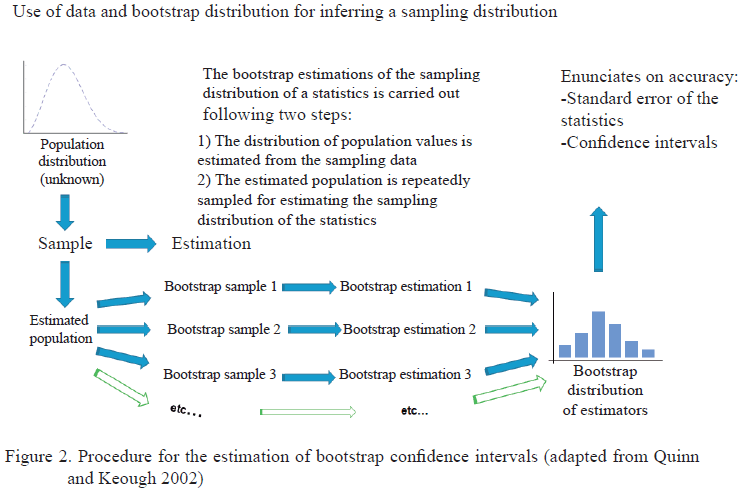
<p align="justify" class="Cuerpodetexto" style="text-indent:0in;"><span style="font-family:'Verdana','sans-serif'; font-size:10.0pt; ">For example, Card B(15) = 7.8 x 10<sup>7</sup>; Card B    (20) = 6.9 x 10<sup>10</sup>.</span></p>     <p align="justify" class="Cuerpodetexto" style="text-indent:0in;"><span style="font-family:'Verdana','sans-serif'; font-size:10.0pt; ">In the bootstrap inference, combined to the mistake  committed using a particular M sample for representing the population, a second  mistake is made by not listing completely all bootstrap samples.&nbsp; This latter mistake can be controlled making  a sufficiently large number of bootstrap repetitions.</span></p>     <p align="justify" class="Cuerpodetexto" style="text-indent:0in;"><span style="font-family:'Verdana','sans-serif'; font-size:10.0pt; ">At first the bootstrap method can be seen as an analogy in  which the estimation method is based at times. If F is the distribution of the  population that generated a random sample of size n, then the estimator T and  its sampling distribution G (T) can be considered as F functions.&nbsp; Efron suggested that it is possible to  substitute F by a consistent estimation </span><em><span style="font-family:'Calibri','sans-serif'; font-size:10.0pt; ">&#518;</span></em><span style="font-family:'Verdana','sans-serif'; font-size:10.0pt; "> This  estimated distribution </span><em><span style="font-family:'Calibri','sans-serif'; font-size:10.0pt; ">&#518;</span></em><span style="font-family:'Verdana','sans-serif'; font-size:10.0pt; "> is a function of empirical distribution assigning the  sample probability, l/n, to each observation in the random sample.&nbsp; Finally what Efron made was to estimate the  sampling distribution G(T) with the bootstrap distribution of the statistical  values G*(</span><em><span style="font-family:'Calibri','sans-serif'; font-size:10.0pt; ">&#518;</span></em><span style="font-family:'Verdana','sans-serif'; font-size:10.0pt; ">) by Monte Carlo simulation.</span></p>     <p align="justify" class="Cuerpodetexto" style="text-indent:0in;"><em><span style="font-family:'Verdana','sans-serif'; font-size:10.0pt; ">Estimation by bootstrap confidence intervals</span></em><span style="font-family:'Verdana','sans-serif'; font-size:10.0pt; ">. From its origin, one of the main research tasks in  bootstrapping has been the development of methods for calculating valid  confidence limits for population parameters (<a href="/img/revistas/cjas/v50n1/f0204116.gif">figure 2</a>). These methods are of  very diverse kinds and are mainly differentiated by the assumptions made on the  estimators and simulation algorithms for obtaining bootstrap samples.&nbsp; Manly (2007) describes some of these  methods.&nbsp; The most popular are:</span></p>     
<p align="justify" class="Cuerpodetexto" style="text-indent:0in;"><span style="font-family:'Verdana','sans-serif'; font-size:10.0pt; ">-Standard bootstrap (normal method): It suppose that the  bootstrap estimator has an approximately normal distribution and the bootstrap  re-sampling gives a good approximation of the statistical standard error of  interest.</span></p>     <p align="justify" class="Cuerpodetexto" style="text-indent:0in;"><span style="font-family:'Verdana','sans-serif'; font-size:10.0pt; ">-First percentile method (percentile method of Efron  (l979). The limits of 100 (1 &ndash; &alpha;)% are determined with values of the bootstrap  distribution of the statistics of interest occupied by the percentiles 100  (&alpha;/2)% and 100 (1 &ndash; &alpha;/2)%. In this procedure it is supposed that there is a  monotonous transformation of estimator values distributed normally.</span></p>     <p align="justify" class="Cuerpodetexto" style="text-indent:0in;"><span style="font-family:'Verdana','sans-serif'; font-size:10.0pt; ">-</span><span style="font-family:'Verdana','sans-serif'; font-size:10.0pt; ">Second percentile method  (Hall&rsquo;s method).&nbsp; It is based on  generating the distribution of the difference between the bootstrap estimation  and the estimation of the parameter calculated with the original&nbsp; sample. </span></p>     <p align="justify" class="Cuerpodetexto" style="text-indent:0in;"><span style="font-family:'Verdana','sans-serif'; font-size:10.0pt; ">-</span><span style="font-family:'Verdana','sans-serif'; font-size:10.0pt; ">Percentile with corrected  bias. It corrects any bias arising from applying the first percentile method,  making the median of the estimator distribution be equal to the mean. The  algorithm of the percentile method with corrected bias uses a more complex  algorithm than the first percentile since in the confidence limits takes into  account the proportion of times that the bootstrap estimation is higher than  the estimation of the parameter using an original sample. </span></p>     <p align="justify" class="Cuerpodetexto" style="text-indent:0in;"><span style="font-family:'Verdana','sans-serif'; font-size:10.0pt; ">-</span><span style="font-family:'Verdana','sans-serif'; font-size:10.0pt; ">Percentile with correction  by accelerated bias.&nbsp; Proposed by Efron  and Tibshirani (1986), it assumes that there is also a monotonous value&nbsp; transformation of the estimator normally  distributed, but the mean and standard error of this distribution are linear  functions of the transformation itself as could happen when the standard error  of the distribution varies with the mean.</span></p>     ]]></body>
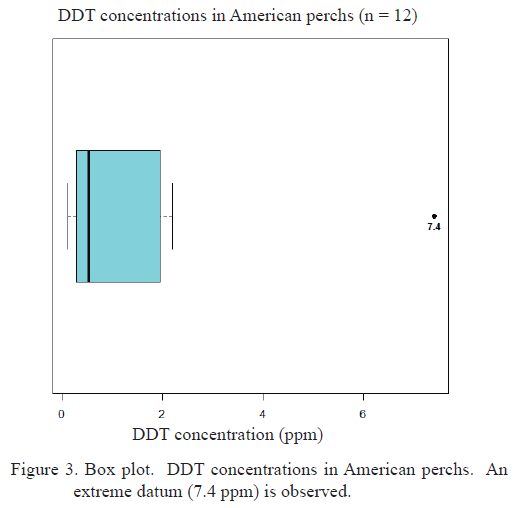
<body><![CDATA[<p align="justify" class="Cuerpodetexto" style="text-indent:0in;"><span style="font-family:'Verdana','sans-serif'; font-size:10.0pt; ">-Bootstrap-t. It uses a t&nbsp; pivotal  statistic calculated for each bootstrap sample.&nbsp;  The calculations in this algorithm are more intensive, requiring  calculating the parameter estimators, as of its standard error, for each  bootstrap sample (this standard error could be calculated by jacknife) </span></p>     <p align="justify" class="Cuerpodetexto" style="text-indent:0in;"><em><span style="font-family:'Verdana','sans-serif'; font-size:10.0pt; ">Bootstrap  confidence limits for the mean</span></em><span style="font-family:'Verdana','sans-serif'; font-size:10.0pt; ">. In some  statistical texts (e.g. Sokal and Rohlf 2012) is presented the formula: <em>EE</em><sub>sampling  median</sub>= 1.253 &sigma;/ &radic;<em>n</em>, </span></p>     <p align="justify" class="Cuerpodetexto" style="text-indent:0in;"><span style="font-family:'Verdana','sans-serif'; font-size:10.0pt; ">where &alpha; is the population standard deviation of a continuous random variable, Y.&nbsp; If &alpha; is not known, then its substitution with  the sampling standard deviation would only be valid for large samples and  normal distributions.&nbsp; But it could occur  that the distribution of variables of the random variable Y does not follow a  normal one, making invalid the application of the estimator of the median  standard error, and thus, the calculation of the confidence limits for this  parameter. In the case of Y variables, positively biased, that follow a  distribution log normal, an alternative method can be used involving taking Y,  = log (Y) as variable approximately normal for calculating the conventional  confidence interval based on the t of Student for Y, mean.&nbsp; The median parametric confidence interval  will be obtained by applying the transformation backwards the interval for this  mean. Given the restrictions for applying these parametric methods of median  estimation, the use of non-parametric methods is generally chosen.&nbsp; The most common are:</span></p>     <p align="justify" class="Cuerpodetexto" style="text-indent:0in;"><span style="font-family:'Verdana','sans-serif'; font-size:10.0pt; ">1.  Quantiles of binomial distribution with percentile p = 0.5. These quantiles are  the same used for the median sign test  (Hollander and Wolfe 2011).&nbsp; Given a  confidence level (1 &ndash; &alpha;) x 100%, the binomial probabilities supply inferior  (x&rsquo;) and superior (x) critical values, corresponding to half the significance  level, &alpha;/2. These critical values correspond to <em>R</em><sub>Inf</sub><em>=x&rsquo;</em>+1  and  <em>R</em><sub>inf</sub>= n-<em>x&rsquo;=x</em> ranges of the arranged sample so as the  values of the variable occupying those places, <em>y<span style="position:relative; top:3.0pt; ">R</span></em><sub>inf</sub>&nbsp;&nbsp;and <em>y<span style="position:relative; top:2.0pt; ">R</span></em><sub>inf</sub>will  constitute the confidence limits of (l &ndash; &alpha;) x 100 % for the mean. This method  is adequate for small samples, that is, n &le; 20 (Helsel &amp; Hirsch 2002). </span></p>     <p align="justify" class="Cuerpodetexto" style="text-indent:0in;"><span style="font-family:'Verdana','sans-serif'; font-size:10.0pt; ">2. Approximation of the method of binomial quantiles to  the normal distribution. It is preferably applied for large samples (n &gt; 20)  and it is based on critical values of the standard normal z<sub>&alpha;/2</sub>. The  confidence limits for the median </span><em><span style=" letter-spacing:-.1pt; font-family:'Verdana','sans-serif'; font-size:10.0pt; ">y</span></em><em><span style=" position:relative; top:3.0pt; font-family:'Verdana','sans-serif'; font-size:10.0pt; ">R</span></em><sub><span style="font-family:'Verdana','sans-serif'; font-size:10.0pt; ">inf</span></sub><span style=" letter-spacing:-.05pt; font-family:'Verdana','sans-serif'; font-size:10.0pt; ">&nbsp;</span><span style="font-family:'Verdana','sans-serif'; font-size:10.0pt; ">&nbsp;and <em>yR</em><sub>inf</sub></span><span style="font-family:'Verdana','sans-serif'; font-size:10.0pt; ">&nbsp;will be those  values of the arranged sample occupying places offered by the following  expressions, conveniently rounded off to the closer whole numbers:</span></p>     <p align="justify" class="Cuerpodetexto" style="text-indent:0in;"><span style="font-family:'Verdana','sans-serif'; font-size:10.0pt; ">&nbsp;</span><em><span style="font-family:'Verdana','sans-serif'; font-size:10.0pt; ">R</span></em><sub><span style="font-family:'Verdana','sans-serif'; font-size:10.0pt; ">inf</span></sub><span style="font-family:'Verdana','sans-serif'; font-size:10.0pt; ">=(<em>n-z<sub>&alpha;/2</sub>&radic;n</em>)/2 y <em>R</em><sub>inf</sub>=(<em>n+z<sub>&alpha;/2</sub>&radic;n</em>)/2+1</span><span style="font-family:'Verdana','sans-serif'; font-size:10.0pt; "> </span></p>     <p align="justify" class="Cuerpodetexto" style="text-indent:0in;"><span style="font-family:'Verdana','sans-serif'; font-size:10.0pt; ">3. Method based on the range test with Wilcoxon sign.&nbsp; It is based on the equivalence of the  statistics T<sup>+</sup> of this test with the average number of Walsh  positive.&nbsp; Walsh averages for a sample {<em>y<sub>1</sub>,  y<sub>2</sub>&hellip;,y<sub>n</sub></em>} constitute a set of n (n + 1)/2, numbers </span><em><span style="font-family:'Verdana','sans-serif'; font-size:10.0pt; ">W<sub>ij</sub>=(y<sub>i</sub>+y<sub>j</sub>)</span></em><span style="font-family:'Verdana','sans-serif'; font-size:10.0pt; ">/2,<em>i&lt;j</em></span><span style="font-family:'Verdana','sans-serif'; font-size:10.0pt; ">.  When Walsh averages are arranged from lesser to greater, </span><em><span style="font-family:'Verdana','sans-serif'; font-size:10.0pt; ">W<sub>(1)</sub>,W<sub>(2)</sub>,&hellip;&hellip;,W<sub>(n(n+1)</sub></span></em><sub><span style="font-family:'Verdana','sans-serif'; font-size:10.0pt; ">/2)</span></sub><span style="font-family:'Verdana','sans-serif'; font-size:10.0pt; "> </span><span style="font-family:'Verdana','sans-serif'; font-size:10.0pt; ">, the confidence limits can be calculated following the  same procedure of the quantile method of the binomial distribution. The mean of  the Walsh averages can be used as estimator (from Hodges-Lehmann) of the  distribution median from where the sample was taken under the supposition that  such distribution was symmetric.&nbsp; If the  distribution is not symmetric, then the estimator will be denominated the  pseudo-median.</span></p>     <p align="justify" class="Cuerpodetexto" style="text-indent:0in;"><span style="font-family:'Verdana','sans-serif'; font-size:10.0pt; ">4. Non-parametric bootstrap. This method is described with  the following example: <a href="/img/revistas/cjas/v50n1/f0304116.gif">Figure 3</a> shows the values of DDT concentration, measured  in 12 specimens of the American perch, sampled in the Tennessee River (Sincich  1993). In view of the positive bias observed in the sample of DDT  concentrations, it is reasonable to use the median as summary measurement of  the value distribution center of the variable Y = &ldquo;DDT concentration&rdquo; and  presenting a confidence interval for the median for inference purposes.</span></p>     
<p align="justify" class="Cuerpodetexto" style="text-indent:0in;"><span style=" letter-spacing:.1pt; font-family:'Verdana','sans-serif'; font-size:10.0pt; ">In total, nine methods were applied. First, the backwards  transformation of the confidence interval was utilized for the median of log  (Y), under the supposition that Y is distributed log-normally. For avoiding the  possibility of assuming any distribution, for the variable Y it was also  estimated the confidence interval for the median based on non-parametric  methods.&nbsp; Methods 1-3 were applied which  were described in the previous section and also the bootstrap (4) was employed,  according to the procedure illustrated in <a href="/img/revistas/cjas/v50n1/f0204116.gif">figure 2</a> for inferring the sampling  distribution of the sampling median based on the examined sample. For this, the  bootstrap distribution (empirical) of the median estimations was generated by  simulation, in which each median was estimated from the random selection with  substitution of the DDT values for obtaining later the median non-parametric  bootstrap confidence limits.&nbsp; The  estimation methods used were five:&nbsp;  Standard or Normal, First Percentile Method, Second Percentile Method  (also called &ldquo;Ordinary&rdquo;), Percentile of Correction by Accelerated Bias and  Bootstrap-t.&nbsp; The calculations were made  with functions of the R program (R Core Team 2015) and the &ldquo;simpleboot&rdquo; package  (Peng 2008)</span><font size="2" face="Verdana, Arial, Helvetica, sans-serif">.</font></p>     
<p align="justify">&nbsp;</p>     ]]></body>
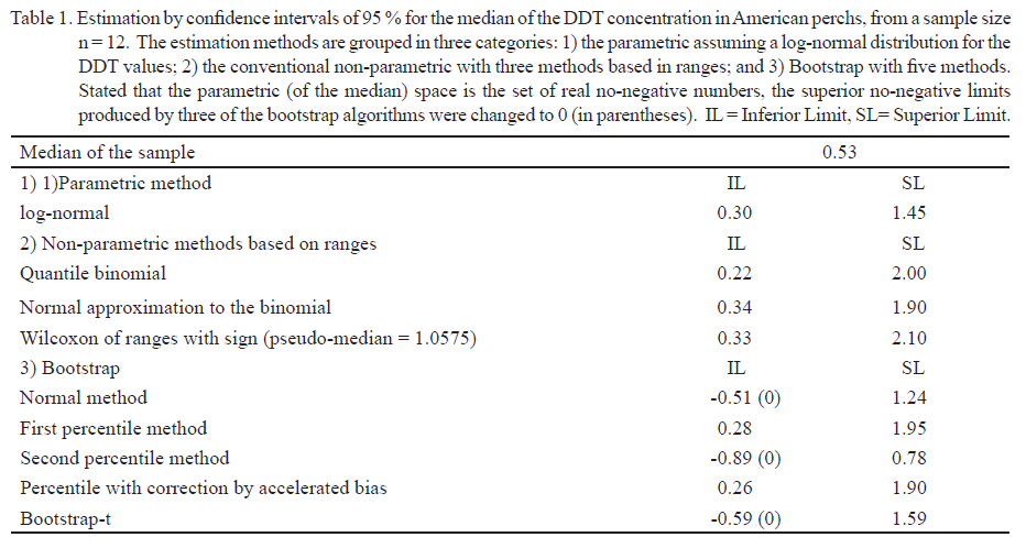
<body><![CDATA[<p align="justify"><font size="2" face="Verdana, Arial, Helvetica, sans-serif"><b><font size="3">RESULTS AND DISCUSSION</font></b></font></p>     <p align="justify" class="Cuerpodetexto" style="text-indent:0in;"><span style=" letter-spacing:.1pt; font-family:'Verdana','sans-serif'; font-size:10.0pt; ">Results from the estimations by intervals for the median  concentration of DDT with the use of the nine methods described in the section  &ldquo;Confidence limits for the median&rdquo;, are set out in <a href="/img/revistas/cjas/v50n1/t0104116.gif">table 1</a>.&nbsp; It can be noticed that the normal bootstrap  method, the second percentile method and the bootstrap-t produce confidence  intervals whose lower limits are negative.&nbsp;  However, the parametric space of the median is no-negative since the DDT  concentration values are also no-negative. Therefore, such lower limits must be  changed to 0.&nbsp; Under this criterion, the  smallest confidence interval is generated by the second percentile method.&nbsp; A graphic summary of the estimated confidence  limits with this method is shown in <a href="/img/revistas/cjas/v50n1/f0404116.gif">figure 4</a>.</span> </p>     
<p align="justify" class="Cuerpodetexto" style="text-indent:0in;"><span style=" letter-spacing:.2pt; font-family:'Verdana','sans-serif'; font-size:10.0pt; ">Which is the best method (parametric or non-parametric)  for estimating confidence intervals for the median? From the set of data  analyzed it can be discerned that the functioning of the different estimation  methods by intervals for the median is very variable.&nbsp; Surprisingly, the parametric interval exceeds  in its accuracy the non-parametric methods.&nbsp;  In addition, the percentile methods and the percentile with correction  by accelerated bias estimate bootstrap intervals for the median similar to  those calculated with conventional non-parametric methods. It also attracts  attention the bootstrap intervals producing negative limits, in spite that the  parametric space is the set of real no-negative numbers.&nbsp; This brings about the need of modifying the  result for obtaining sensible results. What has been observed with this small  example of median estimation is recurrent in statistics: there is no clear  &ldquo;winner&rdquo; as best estimator of some parameter especially when the sample is  relatively small.&nbsp; This also applies, in  particular, to the non-parametric bootstrap methods.&nbsp; As Manly (2007) indicates it is not possible  anticipating in general which of the bootstrap methods allows obtaining better  estimations of a parameter.&nbsp; The bright  side regarding the use of the bootstrap is that it increases the options for  obtaining sensible estimations by parameter intervals of interest in  practically any area of applied sciences.</span><span style="font-family:'Verdana','sans-serif'; font-size:10.0pt; "> </span></p>     <p align="justify" class="Cuerpodetexto" style="text-indent:0in;"><span style="font-family:'Verdana','sans-serif'; font-size:10.0pt; ">Bootstrap has been used for estimating standard errors and  creating confidence intervals of parameters of only one sample, but the  procedure can be extended for the estimation of parameters of two o more  samples and for bootstrap hypothesis tests.&nbsp;  For example, for median comparison of two samples a test statistics (based  on the medians of each sample and the overall median) can be selected so as its  value is comparable to a bootstrap distribution for which the null hypothesis  is true.&nbsp; An alternative approach implies  adjusting the sampling values through the residues (the difference between each  datum and the sample median to which it belongs).&nbsp; A description of these two approaches of  bootstrap tests for two samples can be seen in Manly (2007).&nbsp; In this same reference there is an extensive  list of bootstrap application methods in biological sciences, especially in  Ecology, Genetics, Evolution, Community Ecology and Environmental    Studies.</span><span style="font-family:'Verdana','sans-serif'; font-size:10.0pt; "> </span></p>     <p align="justify" class="Cuerpodetexto" style="text-indent:0in;"><span style="font-family:'Verdana','sans-serif'; font-size:10.0pt; ">In the field of agricultural sciences bootstrap is less  used but not for that is less important. A recent example is the work of  Cubayano <em>et al.</em> (2015) who assessed the accuracy of prediction models of  reproductive values in beef cattle.&nbsp;  These authors used bootstrap for comparing the prediction reliabilities  of reproductive values of some complex traits.&nbsp;  Another recent paper is that of Narin&ccedil; <em>et al.</em> (2015) comparing  two median estimations of three parameters characterizing the color of egg  yolks: one was the conventional median estimation and the other the bootstrap  estimation.&nbsp; This type of study, in which  the conventional parametric methods and the bootstrap are applied and compared,  is frequent in animal science. Hence, in the determination of reference  intervals of physiological parameters in animals, the bootstrap confidence  intervals seem to have better performance under conditions where the  conventional parametric methods are not applicable. Examples of these studies  of reference intervals are those carried out by Bennett <em>et al.</em> (2006)  with physiological parameters in greyhounds and by Cooper <em>et al.</em> (2014)  with biochemical and hematological parameters in pigs.&nbsp; In other estimation problems, as the  determination of the sample size in studies searching for the optimization of  the number of samples, the bootstrap method has shown to be a good alternative  (see Bravo-Iglesias 2010 and Bravo-Iglesias <em>et al.</em> 2013).</span></p>     <p align="justify" class="Cuerpodetexto" style="text-indent:0in;"><span style="font-family:'Verdana','sans-serif'; font-size:10.0pt; ">The strategy of realizing statistical bootstrap tests for  solving problems that have to do with the analysis of variance of one or  various factors, the multiple regressions or the survival has been used in  numerous agricultural and animal sciences investigations. In the majority of  the cases, the bootstrap is utilized for proving the fit goodness of models or  its selection (Casellas <em>et al.</em> 2006, Sahinler and Karakok 2008 and  Tarr&eacute;s <em>et al.</em> 2011, Faridi <em>et al.</em> 2014 and Rodr&iacute;guez <em>et al.</em> 2013).&nbsp; Additionally, it has been employed  for the control of error rates Type I in multiple tests (Meuwissen and Goddard  2004 on false discovery rates in the comparison of two treatments affecting the  expressions of a considerable amount of    genes).</span></p>     <p align="justify"><span style=" letter-spacing:.1pt; font-family:'Verdana','sans-serif'; font-size:10.0pt; ">Since  the publication of the classical papers of Efron (1979), the use of bootstrap  has been explosive since many persons have found in the method complete  response to difficult questions.&nbsp; The  most popular bootstrap method is the one having the simplest theoretical bases:  Efron&rsquo;s percentile. The users are more reluctant to use the other methods due  to the sophistication of the supporting theory.&nbsp;  For example, Manly and Navarro (2009) applied bootstrap-t for estimating  the confidence interval for the difference of two medians when the variances are  very different and distributions are very biased and these authors found very  imprecise results.&nbsp; Therefore, the  bootstrap must be utilized careful in situations in which it has not been  thoroughly tested. Theory guarantees that the bootstrap will function well in  certain situations with large samples, but with small samples it is not  possible anticipating if it will operate better or worst (&iexcl;) than the  parametric and conventional non-parametric methods.&nbsp; Prior suggesting the particular utilization  of bootstrap for small samples, it is recommended testing the procedure with  simulated samples. Undoubtedly the bootstrapping applications for confidence  intervals and significance tests will continue developing in the future and  only those methods with clear properties and with computer support for its  operation in standard statistical packages will prevail</span><font size="2" face="Verdana, Arial, Helvetica, sans-serif">.</font></p>      <p align="justify">&nbsp;</p>      <p align="justify"><font size="2" face="Verdana, Arial, Helvetica, sans-serif"><font size="3"><b>REFERENCES</b></font></font></p>     <p align="justify" class="MsoBibliography"><span style=" font-family:'Verdana','sans-serif'; font-size:10.0pt; ">Bennett S.,  Abraham L., Anderson G., Holloway S. &amp; Parry B. 2006. &lsquo;&lsquo;Reference limits  for urinary fractional excretion of electrolytes in adult non-racing Greyhound  dogs&rsquo;&rsquo;. <em>Australian Veterinary Journal</em>, 84 (11), pp. 393&ndash;397, ISSN:  1751-0813, DOI: 10.1111/j.1751-0813.2006.00057.x.</span></p>     ]]></body>
<body><![CDATA[<!-- ref --><p align="justify" class="MsoBibliography"><span style="font-family:'Verdana','sans-serif'; font-size:10.0pt; ">Bravo I. J. A.  2010. </span><em><span style="font-family:'Verdana','sans-serif'; font-size:10.0pt; ">Aplicaci&oacute;n del m&eacute;todo Bootstrap para la estimaci&oacute;n de  par&aacute;metros poblacionales en Parcelas Permanentes de Muestreo y en la modelaci&oacute;n  Matem&aacute;tica en plantaciones de Pinus cubensis Griseb</span></em><span style="font-family:'Verdana','sans-serif'; font-size:10.0pt; ">.  Ph.D. Thesis, Universidad Pinar del R&iacute;o, Cuba.    </span></p>     <p align="justify" class="MsoBibliography"><span style="font-family:'Verdana','sans-serif'; font-size:10.0pt; ">Bravo J., Torres V., Rodr&iacute;guez L., Montalvo  J., Toirac W., Fuentes V. &amp; Rodr&iacute;guez P. 2011. &lsquo;&lsquo;Determinaci&oacute;n del tama&ntilde;o  de muestra en parcelas permanentes de muestreo mediante la aplicaci&oacute;n del  m&eacute;todo bootstrap&rsquo;&rsquo;. </span><em><span style="font-family:'Verdana','sans-serif'; font-size:10.0pt; ">Revista  Forestal Baracoa</span></em><span style="font-family:'Verdana','sans-serif'; font-size:10.0pt; ">, 32 (1), pp.  57&ndash;65, ISSN: 0138-6441.</span></p>     <p align="justify" class="MsoBibliography"><span style="font-family:'Verdana','sans-serif'; font-size:10.0pt; ">Casellas J.  2006. &lsquo;&lsquo;Parametric bootstrap for testing model fitting in the proportional  hazards framework: An application to the survival analysis of Bruna dels  Pirineus beef calves&rsquo;&rsquo;. <em>Journal of Animal Science</em>, 84 (10), pp.  2609&ndash;2616, ISSN: 0021-8812, 1525-3163, DOI: 10.2527/jas.2005-729.</span></p>     <p align="justify" class="MsoBibliography"><span style="font-family:'Verdana','sans-serif'; font-size:10.0pt; ">Cooper C. A.,  Moraes L. E., Murray J. D. &amp; Owens S. D. 2014. &lsquo;&lsquo;Hematologic and  biochemical reference intervals for specific pathogen free 6-week-old  Hampshire-Yorkshire crossbred pigs&rsquo;&rsquo;. <em>Journal of Animal Science and  Biotechnology</em>, 5, p. 5, ISSN: 2049-1891, DOI: 10.1186/2049-1891-5-5.</span></p>     <p align="justify" class="MsoBibliography"><span style="font-family:'Verdana','sans-serif'; font-size:10.0pt; ">Cuyabano B. C.  D., Su G., Rosa G. J. M., Lund M. S. &amp; Gianola D. 2015. &lsquo;&lsquo;Bootstrap study  of genome-enabled prediction reliabilities using haplotype blocks across Nordic  Red cattle breeds&rsquo;&rsquo;. <em>Journal of Dairy Science</em>, 98 (10), pp. 7351&ndash;7363,  ISSN: 0022-0302, DOI: 10.3168/jds.2015-9360.</span></p>     <p align="justify" class="MsoBibliography"><span style="font-family:'Verdana','sans-serif'; font-size:10.0pt; ">Efron B. 1979.  &lsquo;&lsquo;Bootstrap Methods: Another Look at the Jackknife&rsquo;&rsquo;. <em>The Annals of  Statistics</em>, 7 (1), pp. 1&ndash;26, ISSN: 0090-5364, 2168-8966, DOI:  10.1214/aos/1176344552, MR: MR515681Zbl: 0406.62024.</span></p>     <!-- ref --><p align="justify" class="MsoBibliography"><span style="font-family:'Verdana','sans-serif'; font-size:10.0pt; ">Efron B. &amp;  Tibshirani R. J. 1994. <em>An Introduction to the Bootstrap</em>. CRC Press, 456  p., ISBN: 978-0-412-04231-7.    </span></p>     <p align="justify" class="MsoBibliography"><span style="font-family:'Verdana','sans-serif'; font-size:10.0pt; ">Faridi A.,  Golian A., Mousavi A. H. &amp; France J. 2013. &lsquo;&lsquo;Bootstrapped neural network  models for analyzing the responses of broiler chicks to dietary protein and  branched chain amino acids&rsquo;&rsquo;. <em>Canadian Journal of Animal Science</em>, 94  (1), pp. 79&ndash;85, ISSN: 0008-3984, DOI: 10.4141/cjas2013-078.</span></p>     ]]></body>
<body><![CDATA[<!-- ref --><p align="justify" class="MsoBibliography"><span style="font-family:'Verdana','sans-serif'; font-size:10.0pt; ">Manly B. F. J.  2006. <em>Randomization, Bootstrap and Monte Carlo Methods in Biology</em>. 3rd  ed., Boca Raton, FL: Chapman and Hall/CRC, 480 p., ISBN: 978-1-58488-541-2.    </span></p>     <p align="justify" class="MsoBibliography"><span style="font-family:'Verdana','sans-serif'; font-size:10.0pt; ">Manly B. F. J. &amp; Navarro J. 2009. </span><span style="font-family:'Verdana','sans-serif'; font-size:10.0pt; ">&lsquo;&lsquo;Bootstrap Tests and Confidence Intervals for  Non-Normal Data&rsquo;&rsquo;. In: Ronja F. (ed.), <em>Neue Methoden der Biometrie: Beitr&auml;ge  des 55. Biometrischen Kolloquiums an der Leibniz-Universit&auml;t Hannover 2009</em>,  Hannover, Germany: Institut f&uuml;r Biostatistik, p. 76.</span></p>     <p align="justify" class="MsoBibliography"><span style="font-family:'Verdana','sans-serif'; font-size:10.0pt; ">Meuwissen T.  H. E. &amp; Goddard M. E. 2004. &lsquo;&lsquo;Bootstrapping of gene-expression data  improves and controls the false discovery rate of differentially expressed  genes&rsquo;&rsquo;. <em>Genetics, selection, evolution: GSE</em>, 36 (2), pp. 191&ndash;205, ISSN:  0999-193X, DOI: 10.1051/gse:2003058, PMID: 15040898PMCID: PMC2697185.</span></p>     <p align="justify" class="MsoBibliography"><span style="font-family:'Verdana','sans-serif'; font-size:10.0pt; ">Narin&ccedil; D.,  Ayg&uuml;n A., K&uuml;&ccedil;&uuml;k&ouml;nder H., Aksoy T. &amp; G&Uuml;RCAN E. K. 2015. &lsquo;&lsquo;An Application of  Bootstrap Technique in Animal Science: Egg Yolk Color Sample&rsquo;&rsquo;. <em>Kafkas  &Uuml;niversitesi Veteriner Fak&uuml;ltesi Dergisi</em>, 21 (5), pp. 631&ndash;637, ISSN:  1300-6045, 1309-2251.</span></p>     <!-- ref --><p align="justify" class="MsoBibliography"><span style="font-family:'Verdana','sans-serif'; font-size:10.0pt; ">Peng R. D.  2008. <em>Simpleboot: Simple Bootstrap Routines. R package.</em> version 1.1-3,  Available:  &lt;<a href="https://cran.itam.mx/bin/windows/contrib/3.2/simpleboot_1.1-3.zip" target="_blank">https://cran.itam.mx/bin/windows/contrib/3.2/simpleboot_1.1-3.zip</a>&gt;    .</span></p>     <p align="justify" class="MsoBibliography"><span style="font-family:'Verdana','sans-serif'; font-size:10.0pt; ">Quenouille M.  H. 1949. &lsquo;&lsquo;Approximate tests of correlation in time-series 3&rsquo;&rsquo;. <em>Mathematical  Proceedings of the Cambridge Philosophical Society</em>, 45 (03), pp. 483&ndash;484,  ISSN: 1469-8064, DOI: 10.1017/S0305004100025123.</span></p>     <p align="justify" class="MsoBibliography"><span style="font-family:'Verdana','sans-serif'; font-size:10.0pt; ">Quenouille M.  H. 1956. &lsquo;&lsquo;Notes on Bias in Estimation&rsquo;&rsquo;. <em>Biometrika</em>, 43 (3/4), pp.  353&ndash;360, ISSN: 0006-3444, DOI: 10.2307/2332914.</span></p>     <!-- ref --><p align="justify" class="MsoBibliography"><span style="font-family:'Verdana','sans-serif'; font-size:10.0pt; ">Quinn G. P.  &amp; Keough M. J. 2002. <em>Experimental Design and Data Analysis for  Biologists</em>. Cambridge, New York: Cambridge University Press, 560 p., ISBN:  978-0-521-00976-8.    </span></p>     <!-- ref --><p align="justify" class="MsoBibliography"><span style="font-family:'Verdana','sans-serif'; font-size:10.0pt; ">R Core Team.  2015. <em>R: A language and environment for statistical computing</em>. Vienna,  Austria: R&nbsp;&nbsp; Foundation for Statistical  Computing, Available: &lt;<a href="https://www.R-project.org/" target="_blank">https://www.R-project.org/</a>&gt;    .</span></p>     <p align="justify" class="MsoBibliography"><span style="font-family:'Verdana','sans-serif'; font-size:10.0pt; ">Rodr&iacute;guez L., Larduet R., Mart&iacute;nez R. O.,  Torres V., Herrera M., Medina Y. &amp; Noda A. C. 2013. &lsquo;&lsquo;Modelaci&oacute;n de la  din&aacute;mica de acumulaci&oacute;n de biomasa en <em>Pennisetum purpureum</em> vc. king  grass en el occidente de Cuba&rsquo;&rsquo;. <em>Revista Cubana de Ciencia Agr&iacute;cola</em>, 47  (2), pp. 119&ndash;124, ISSN: 2079-3480.</span></p>     <p align="justify" class="MsoBibliography"><span style="font-family:'Verdana','sans-serif'; font-size:10.0pt; ">Sahinler S. &amp; Karakok S. G. 2008. </span><span style="font-family:'Verdana','sans-serif'; font-size:10.0pt; ">&lsquo;&lsquo;Bootstrap and Jackknife Parameter Estimation of the  Models Fitting to Lactation Milk Yield (2x305) on Calving Age&rsquo;&rsquo;. <em>Journal of  Applied Animal Research</em>, 34 (1), pp. 39&ndash;44, ISSN: 0971-2119, DOI:  10.1080/09712119.2008.9706937.</span></p>     <!-- ref --><p align="justify" class="MsoBibliography"><span style="font-family:'Verdana','sans-serif'; font-size:10.0pt; ">Sincich T.  1993. <em>Statistics by Example</em>. 5th ed., New York: Dellen Pub Co, 1024 p.,  ISBN: 978-0-02-410981-1.    </span></p>     <p align="justify" class="MsoBibliography"><span style="font-family:'Verdana','sans-serif'; font-size:10.0pt; ">Tarr&eacute;s J., Fina M., Varona L. &amp;  Piedrafita J. 2011. </span><span style="font-family:'Verdana','sans-serif'; font-size:10.0pt; ">&lsquo;&lsquo;Carcass  conformation and fat cover scores in beef cattle: A comparison of threshold  linear models vs grouped data models&rsquo;&rsquo;. <em>Genetics Selection Evolution</em>, 43  (1), pp. 1&ndash;10, ISSN: 1297-9686, DOI: 10.1186/1297-9686-43-16.</span></p>     <p align="justify"><span style="font-family:'Verdana','sans-serif'; font-size:10.0pt; ">Tukey J. W. 1958. &lsquo;&lsquo;Bias  and confidence in not quite large samples&rsquo;&rsquo;. </span><em><span style="font-family:'Verdana','sans-serif'; font-size:10.0pt; ">The Annals of Mathematical Statistics</span></em><span style="font-family:'Verdana','sans-serif'; font-size:10.0pt; ">, 29 (2), pp. 614&ndash;623,  ISSN: 0003-4851, DOI: 10.1214/aoms/1177706647.</span> </p>     <p align="justify">&nbsp;</p>     ]]></body>
<body><![CDATA[<p align="justify">&nbsp;</p>     <p align="justify"><font size="2" face="Verdana, Arial, Helvetica, sans-serif">Received: November 25, 2015    <br>   Accepted: March 11, 2016</font></p>     <p align="justify">&nbsp;</p>     <p align="justify">&nbsp;</p>     <p align="justify"><font size="2" face="Verdana, Arial, Helvetica, sans-serif"><i>J. A. Navarro Alberto,</i> Departamento de Ecología Tropical Campus de Ciencias Biológicas y Agropecuarias Universidad Autónoma de Yucatán Km 15.5 Carretera Mérida-Xmatkuil. CP 97315. Mérida, Yucatán, México.    Email: <a href="mailto:jorge.navarro@correo.uady.mx">jorge.navarro@correo.uady.mx</a></font></p>      ]]></body><back>
<ref-list>
<ref id="B1">
<nlm-citation citation-type="journal">
<person-group person-group-type="author">
<name>
<surname><![CDATA[Bennett]]></surname>
<given-names><![CDATA[S.]]></given-names>
</name>
<name>
<surname><![CDATA[Abraham]]></surname>
<given-names><![CDATA[L.]]></given-names>
</name>
<name>
<surname><![CDATA[Anderson]]></surname>
<given-names><![CDATA[G.]]></given-names>
</name>
<name>
<surname><![CDATA[Holloway]]></surname>
<given-names><![CDATA[S.]]></given-names>
</name>
<name>
<surname><![CDATA[Parry]]></surname>
<given-names><![CDATA[B.]]></given-names>
</name>
</person-group>
<article-title xml:lang="nd"><![CDATA[Reference limits for urinary fractional excretion of electrolytes in adult non-racing Greyhound dogs]]></article-title>
<source><![CDATA[Australian Veterinary Journal]]></source>
<year>2006</year>
<volume>84</volume>
<numero>11</numero>
<issue>11</issue>
<page-range>393-397</page-range></nlm-citation>
</ref>
<ref id="B2">
<nlm-citation citation-type="book">
<person-group person-group-type="author">
<name>
<surname><![CDATA[Bravo]]></surname>
<given-names><![CDATA[I. J. A.]]></given-names>
</name>
</person-group>
<source><![CDATA[Aplicación del método Bootstrap para la estimación de parámetros poblacionales en Parcelas Permanentes de Muestreo y en la modelación Matemática en plantaciones de Pinus cubensis Griseb]]></source>
<year>2010</year>
<publisher-loc><![CDATA[Cuba ]]></publisher-loc>
<publisher-name><![CDATA[Universidad Pinar del Río]]></publisher-name>
</nlm-citation>
</ref>
<ref id="B3">
<nlm-citation citation-type="journal">
<person-group person-group-type="author">
<name>
<surname><![CDATA[Bravo]]></surname>
<given-names><![CDATA[J.]]></given-names>
</name>
<name>
<surname><![CDATA[Torres]]></surname>
<given-names><![CDATA[V.]]></given-names>
</name>
<name>
<surname><![CDATA[Rodríguez]]></surname>
<given-names><![CDATA[L.]]></given-names>
</name>
<name>
<surname><![CDATA[Montalvo]]></surname>
<given-names><![CDATA[J.]]></given-names>
</name>
<name>
<surname><![CDATA[Toirac]]></surname>
<given-names><![CDATA[W.]]></given-names>
</name>
<name>
<surname><![CDATA[Fuentes]]></surname>
<given-names><![CDATA[V.]]></given-names>
</name>
<name>
<surname><![CDATA[Rodríguez]]></surname>
<given-names><![CDATA[P.]]></given-names>
</name>
</person-group>
<article-title xml:lang="nd"><![CDATA[Determinación del tamaño de muestra en parcelas permanentes de muestreo mediante la aplicación del método bootstrap]]></article-title>
<source><![CDATA[Revista Forestal Baracoa]]></source>
<year>2011</year>
<volume>32</volume>
<numero>1</numero>
<issue>1</issue>
<page-range>57-65</page-range></nlm-citation>
</ref>
<ref id="B4">
<nlm-citation citation-type="journal">
<person-group person-group-type="author">
<name>
<surname><![CDATA[Casellas]]></surname>
<given-names><![CDATA[J.]]></given-names>
</name>
</person-group>
<article-title xml:lang="nd"><![CDATA[Parametric bootstrap for testing model fitting in the proportional hazards framework: An application to the survival analysis of Bruna dels Pirineus beef calves]]></article-title>
<source><![CDATA[Journal of Animal Science]]></source>
<year>2006</year>
<volume>84</volume>
<numero>10</numero>
<issue>10</issue>
<page-range>2609-2616</page-range></nlm-citation>
</ref>
<ref id="B5">
<nlm-citation citation-type="journal">
<person-group person-group-type="author">
<name>
<surname><![CDATA[Cooper]]></surname>
<given-names><![CDATA[C. A.]]></given-names>
</name>
<name>
<surname><![CDATA[Moraes]]></surname>
<given-names><![CDATA[L. E.]]></given-names>
</name>
<name>
<surname><![CDATA[Murray]]></surname>
<given-names><![CDATA[J. D.]]></given-names>
</name>
<name>
<surname><![CDATA[Owens]]></surname>
<given-names><![CDATA[S. D.]]></given-names>
</name>
</person-group>
<article-title xml:lang="nd"><![CDATA[Hematologic and biochemical reference intervals for specific pathogen free 6-week-old Hampshire-Yorkshire crossbred pigs]]></article-title>
<source><![CDATA[Journal of Animal Science and Biotechnology]]></source>
<year>2014</year>
<volume>5</volume>
<page-range>5</page-range></nlm-citation>
</ref>
<ref id="B6">
<nlm-citation citation-type="journal">
<person-group person-group-type="author">
<name>
<surname><![CDATA[Cuyabano]]></surname>
<given-names><![CDATA[B. C. D.]]></given-names>
</name>
<name>
<surname><![CDATA[Su]]></surname>
<given-names><![CDATA[G.]]></given-names>
</name>
<name>
<surname><![CDATA[Rosa]]></surname>
<given-names><![CDATA[G. J. M.]]></given-names>
</name>
<name>
<surname><![CDATA[Lund]]></surname>
<given-names><![CDATA[M. S.]]></given-names>
</name>
<name>
<surname><![CDATA[Gianola]]></surname>
<given-names><![CDATA[D.]]></given-names>
</name>
</person-group>
<article-title xml:lang="nd"><![CDATA[Bootstrap study of genome-enabled prediction reliabilities using haplotype blocks across Nordic Red cattle breeds]]></article-title>
<source><![CDATA[Journal of Dairy Science]]></source>
<year>2015</year>
<volume>98</volume>
<numero>10</numero>
<issue>10</issue>
<page-range>7351-7363</page-range></nlm-citation>
</ref>
<ref id="B7">
<nlm-citation citation-type="journal">
<person-group person-group-type="author">
<name>
<surname><![CDATA[Efron]]></surname>
<given-names><![CDATA[B.]]></given-names>
</name>
</person-group>
<article-title xml:lang="nd"><![CDATA[Bootstrap Methods: Another Look at the Jackknife]]></article-title>
<source><![CDATA[The Annals of Statistics]]></source>
<year>1979</year>
<volume>7</volume>
<numero>1</numero>
<issue>1</issue>
<page-range>1-26</page-range></nlm-citation>
</ref>
<ref id="B8">
<nlm-citation citation-type="book">
<person-group person-group-type="author">
<name>
<surname><![CDATA[Efron]]></surname>
<given-names><![CDATA[B.]]></given-names>
</name>
<name>
<surname><![CDATA[Tibshirani]]></surname>
<given-names><![CDATA[R. J.]]></given-names>
</name>
</person-group>
<source><![CDATA[An Introduction to the Bootstrap]]></source>
<year>1994</year>
<page-range>456</page-range><publisher-name><![CDATA[CRC Press]]></publisher-name>
</nlm-citation>
</ref>
<ref id="B9">
<nlm-citation citation-type="journal">
<person-group person-group-type="author">
<name>
<surname><![CDATA[Faridi]]></surname>
<given-names><![CDATA[A.]]></given-names>
</name>
<name>
<surname><![CDATA[Golian]]></surname>
<given-names><![CDATA[A.]]></given-names>
</name>
<name>
<surname><![CDATA[Mousavi]]></surname>
<given-names><![CDATA[A. H.]]></given-names>
</name>
<name>
<surname><![CDATA[France]]></surname>
<given-names><![CDATA[J.]]></given-names>
</name>
</person-group>
<article-title xml:lang="nd"><![CDATA[Bootstrapped neural network models for analyzing the responses of broiler chicks to dietary protein and branched chain amino acids]]></article-title>
<source><![CDATA[Canadian Journal of Animal Science]]></source>
<year>2013</year>
<volume>94</volume>
<numero>1</numero>
<issue>1</issue>
<page-range>79-85</page-range></nlm-citation>
</ref>
<ref id="B10">
<nlm-citation citation-type="book">
<person-group person-group-type="author">
<name>
<surname><![CDATA[Manly]]></surname>
<given-names><![CDATA[B. F. J.]]></given-names>
</name>
</person-group>
<source><![CDATA[Randomization, Bootstrap and Monte Carlo Methods in Biology]]></source>
<year>2006</year>
<edition>3rd</edition>
<page-range>480</page-range><publisher-loc><![CDATA[Boca Raton, FL ]]></publisher-loc>
<publisher-name><![CDATA[Chapman and Hall/CRC]]></publisher-name>
</nlm-citation>
</ref>
<ref id="B11">
<nlm-citation citation-type="book">
<person-group person-group-type="author">
<name>
<surname><![CDATA[Manly]]></surname>
<given-names><![CDATA[B. F. J.]]></given-names>
</name>
<name>
<surname><![CDATA[Navarro]]></surname>
<given-names><![CDATA[J.]]></given-names>
</name>
</person-group>
<article-title xml:lang="nd"><![CDATA[Bootstrap Tests and Confidence Intervals for Non-Normal Data]]></article-title>
<person-group person-group-type="editor">
<name>
<surname><![CDATA[Ronja]]></surname>
<given-names><![CDATA[F.]]></given-names>
</name>
</person-group>
<source><![CDATA[]]></source>
<year>2009</year>
<page-range>76</page-range><publisher-loc><![CDATA[Hannover, Germany ]]></publisher-loc>
<publisher-name><![CDATA[Institut für Biostatistik]]></publisher-name>
</nlm-citation>
</ref>
<ref id="B12">
<nlm-citation citation-type="journal">
<person-group person-group-type="author">
<name>
<surname><![CDATA[Meuwissen]]></surname>
<given-names><![CDATA[T. H. E.]]></given-names>
</name>
<name>
<surname><![CDATA[Goddard]]></surname>
<given-names><![CDATA[M. E.]]></given-names>
</name>
</person-group>
<article-title xml:lang="nd"><![CDATA[Bootstrapping of gene-expression data improves and controls the false discovery rate of differentially expressed genes]]></article-title>
<source><![CDATA[Genetics, selection, evolution: GSE]]></source>
<year>2004</year>
<volume>36</volume>
<numero>2</numero>
<issue>2</issue>
<page-range>191-205</page-range></nlm-citation>
</ref>
<ref id="B13">
<nlm-citation citation-type="journal">
<person-group person-group-type="author">
<name>
<surname><![CDATA[Narinç]]></surname>
<given-names><![CDATA[D.]]></given-names>
</name>
<name>
<surname><![CDATA[Aygün]]></surname>
<given-names><![CDATA[A.]]></given-names>
</name>
<name>
<surname><![CDATA[Küçükönder]]></surname>
<given-names><![CDATA[H.]]></given-names>
</name>
<name>
<surname><![CDATA[Aksoy]]></surname>
<given-names><![CDATA[T.]]></given-names>
</name>
<name>
<surname><![CDATA[GÜRCAN]]></surname>
<given-names><![CDATA[E. K.]]></given-names>
</name>
</person-group>
<article-title xml:lang="nd"><![CDATA[An Application of Bootstrap Technique in Animal Science: Egg Yolk Color Sample]]></article-title>
<source><![CDATA[Kafkas Üniversitesi Veteriner Fakültesi Dergisi]]></source>
<year>2015</year>
<volume>21</volume>
<numero>5</numero>
<issue>5</issue>
<page-range>631-637</page-range></nlm-citation>
</ref>
<ref id="B14">
<nlm-citation citation-type="">
<person-group person-group-type="author">
<name>
<surname><![CDATA[Peng]]></surname>
<given-names><![CDATA[R. D.]]></given-names>
</name>
</person-group>
<source><![CDATA[Simpleboot: Simple Bootstrap Routines. R package.]]></source>
<year>2008</year>
</nlm-citation>
</ref>
<ref id="B15">
<nlm-citation citation-type="journal">
<person-group person-group-type="author">
<name>
<surname><![CDATA[Quenouille]]></surname>
<given-names><![CDATA[M. H.]]></given-names>
</name>
</person-group>
<article-title xml:lang="nd"><![CDATA[Approximate tests of correlation in time-series 3]]></article-title>
<source><![CDATA[Mathematical Proceedings of the Cambridge Philosophical Society]]></source>
<year>1949</year>
<volume>45</volume>
<numero>03</numero>
<issue>03</issue>
<page-range>483-484</page-range></nlm-citation>
</ref>
<ref id="B16">
<nlm-citation citation-type="journal">
<person-group person-group-type="author">
<name>
<surname><![CDATA[Quenouille]]></surname>
<given-names><![CDATA[M. H.]]></given-names>
</name>
</person-group>
<article-title xml:lang="nd"><![CDATA[Notes on Bias in Estimation]]></article-title>
<source><![CDATA[Biometrika]]></source>
<year>1956</year>
<volume>43</volume>
<numero>3/4</numero>
<issue>3/4</issue>
<page-range>353-360</page-range></nlm-citation>
</ref>
<ref id="B17">
<nlm-citation citation-type="book">
<person-group person-group-type="author">
<name>
<surname><![CDATA[Quinn]]></surname>
<given-names><![CDATA[G. P.]]></given-names>
</name>
<name>
<surname><![CDATA[Keough]]></surname>
<given-names><![CDATA[M. J.]]></given-names>
</name>
</person-group>
<source><![CDATA[Experimental Design and Data Analysis for Biologists]]></source>
<year>2002</year>
<page-range>560</page-range><publisher-loc><![CDATA[Cambridge, New York ]]></publisher-loc>
<publisher-name><![CDATA[Cambridge University Press]]></publisher-name>
</nlm-citation>
</ref>
<ref id="B18">
<nlm-citation citation-type="book">
<person-group person-group-type="author">
<name>
<surname><![CDATA[R Core Team]]></surname>
</name>
</person-group>
<source><![CDATA[R: A language and environment for statistical computing]]></source>
<year>2015</year>
<publisher-loc><![CDATA[Vienna, Austria ]]></publisher-loc>
<publisher-name><![CDATA[R Foundation for Statistical Computing]]></publisher-name>
</nlm-citation>
</ref>
<ref id="B19">
<nlm-citation citation-type="journal">
<person-group person-group-type="author">
<name>
<surname><![CDATA[Rodríguez]]></surname>
<given-names><![CDATA[L.]]></given-names>
</name>
<name>
<surname><![CDATA[Larduet]]></surname>
<given-names><![CDATA[R.]]></given-names>
</name>
<name>
<surname><![CDATA[Martínez]]></surname>
<given-names><![CDATA[R. O.]]></given-names>
</name>
<name>
<surname><![CDATA[Torres]]></surname>
<given-names><![CDATA[V.]]></given-names>
</name>
<name>
<surname><![CDATA[Herrera]]></surname>
<given-names><![CDATA[M.]]></given-names>
</name>
<name>
<surname><![CDATA[Medina]]></surname>
<given-names><![CDATA[Y.]]></given-names>
</name>
<name>
<surname><![CDATA[Noda]]></surname>
<given-names><![CDATA[A. C.]]></given-names>
</name>
</person-group>
<article-title xml:lang="nd"><![CDATA[Modelación de la dinámica de acumulación de biomasa en Pennisetum purpureum vc. king grass en el occidente de Cuba]]></article-title>
<source><![CDATA[Revista Cubana de Ciencia Agrícola]]></source>
<year>2013</year>
<volume>47</volume>
<numero>2</numero>
<issue>2</issue>
<page-range>119-124</page-range></nlm-citation>
</ref>
<ref id="B20">
<nlm-citation citation-type="journal">
<person-group person-group-type="author">
<name>
<surname><![CDATA[Sahinler]]></surname>
<given-names><![CDATA[S.]]></given-names>
</name>
<name>
<surname><![CDATA[Karakok]]></surname>
<given-names><![CDATA[S. G.]]></given-names>
</name>
</person-group>
<article-title xml:lang="nd"><![CDATA[Bootstrap and Jackknife Parameter Estimation of the Models Fitting to Lactation Milk Yield (2x305) on Calving Age]]></article-title>
<source><![CDATA[Journal of Applied Animal Research]]></source>
<year>2008</year>
<volume>34</volume>
<numero>1</numero>
<issue>1</issue>
<page-range>39-44</page-range></nlm-citation>
</ref>
<ref id="B21">
<nlm-citation citation-type="book">
<person-group person-group-type="author">
<name>
<surname><![CDATA[Sincich]]></surname>
<given-names><![CDATA[T.]]></given-names>
</name>
</person-group>
<source><![CDATA[Statistics by Example]]></source>
<year>1993</year>
<edition>5th</edition>
<page-range>1024</page-range><publisher-loc><![CDATA[New York ]]></publisher-loc>
<publisher-name><![CDATA[Dellen Pub Co]]></publisher-name>
</nlm-citation>
</ref>
<ref id="B22">
<nlm-citation citation-type="journal">
<person-group person-group-type="author">
<name>
<surname><![CDATA[Tarrés]]></surname>
<given-names><![CDATA[J.]]></given-names>
</name>
<name>
<surname><![CDATA[Fina]]></surname>
<given-names><![CDATA[M.]]></given-names>
</name>
<name>
<surname><![CDATA[Varona]]></surname>
<given-names><![CDATA[L.]]></given-names>
</name>
<name>
<surname><![CDATA[Piedrafita]]></surname>
<given-names><![CDATA[J.]]></given-names>
</name>
</person-group>
<article-title xml:lang="nd"><![CDATA[Carcass conformation and fat cover scores in beef cattle: A comparison of threshold linear models vs grouped data models]]></article-title>
<source><![CDATA[Genetics Selection Evolution]]></source>
<year>2011</year>
<volume>43</volume>
<numero>1</numero>
<issue>1</issue>
<page-range>1-10</page-range></nlm-citation>
</ref>
<ref id="B23">
<nlm-citation citation-type="journal">
<person-group person-group-type="author">
<name>
<surname><![CDATA[Tukey]]></surname>
<given-names><![CDATA[J. W.]]></given-names>
</name>
</person-group>
<article-title xml:lang="nd"><![CDATA[Bias and confidence in not quite large samples]]></article-title>
<source><![CDATA[The Annals of Mathematical Statistics]]></source>
<year>1958</year>
<volume>29</volume>
<numero>2</numero>
<issue>2</issue>
<page-range>614-623</page-range></nlm-citation>
</ref>
</ref-list>
</back>
</article>