


 Servicios personalizados
 Inglés (pdf)
 Articulo en XML
 Referencias del artículo
 Enviar articulo por email
 Citado por SciELO
  Similares en
SciELO
Similares en
SciELO 
 Permalink
Introduction
COVID-19 is a viral disease with many clinical manifestations, among which dermatological manifestations attract attention because of its high incidence of occurrence.1,2,3,4,5) In addition, sometimes signs and symptoms of COVID-19 are dermatological manifestations in patients without respiratory manifestations.6,7) Therefore, at this time of pandemic, it is extremely important for medicine and especially for the specialty of dermatology to have images that allow the diagnosis of diseases.8,9,10,11
Nowadays, the acquisition and processing of medical images constitutes a very important research area. In addition, the reconstruction of medical images has found many applications.8,12 Furthermore, other applications involving image reconstruction are also found in industrial electronics,13,14,15,16 and in machine vision.17
At present, doctors share large volumes of images, many of which are taken and saved for diagnosis. Therefore, doctors need robust technologies for image interpretation and analysis that avoid losses in quality and features, and that facilitate behavioral patterns identification of the human organism that are manifestations of possible contagion of diseases. To do this, medical images need large amounts of bits to be stored, specifically the ones with high resolution. In addition, for their right transmission networks cannot have limited bandwidth. Therefore, the high bandwidth consumption and the growing demand for huge information storage, make it necessary to count on procedures that allow an efficient low bitrate compression of medical images. In this way, it is intended to carry out the fast, efficient transmission of these images.
What was mentioned in the previous paragraph implies carrying out a compression process. In short, the amount of data must be reduced to represent the images of interest under study, eliminating data that do not provide relevant information on the content of those images. Moreover, while the losses due to the degradation of the image are tolerable, what is lost is insignificant compared to what is gained due to the decrease in file size. Thus, the losses due to the degradation of the image are compensated with what is gained by reducing the size of the files that contain them.
In this paper, the Principal Component Analysis (PCA) technique,18,19,20,21,22,23,24,25) is used to carry out the reduction in the dimension of medical images that represent dermatological manifestations in paucisymptomatic patients of COVID-19. The main objective of this paper is to apply PCA to the compression of a set of photos taken of one of the most frequent patterns in COVID-19, the maculopapular or morbilliform pattern, which is characterized by an erythmatopapular rash.26,27,28,29,30 The rationale behind this research is to try to use lossy compression techniques in medical imaging with a view to solve the problem that it is very difficult to study compressed medical images to diagnose a disease. The proposal is to provide means for the reconstruction of medical images in such a way that we do not lose significant qualities or characteristics of the disease, helping doctors to interpret and improve the diagnosis. This also the motivation of this paper.
The objective of this paper is to present a new application of the PCA technique in the field of industrial electronics, aimed at compressing of medical images. In this case, the quasi-periodicity of the first principal components (PCs),26,27,28,29 is used to perform medical image compression. In short, PCs that are considered periodic are replaced by their period plus a trend, and the reconstruction achieved allows to diagnose some skin diseases.
Methods
For the study, we have a set of 20 images of paucisymptomatic COVID-19 patients, with different resolutions and of different parts of their bodies, where dermatological manifestations are shown. Fig. 1 shows a collage of the images under study. In order to obtain reasonable reconstructions of compressed images, they were compressed using the PCA technique.
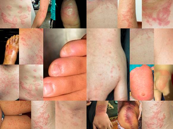
At this point, it is important to mention that to obtain the images, the first thing that was done was to have the authorized consent of each patient, to take the photographs and publish them for scientific research purposes. The photos were taken with the Huawei P30 Lite MAR-LX3A smartphone along with the Magnifier Camera 1.6.0 for Android application. Here, to take the photos, the most recent lesions that are illustrative of the maculopapular pattern were chosen and with good lighting, at a reasonable distance between 50 mm and 105 mm, the photos were taken.
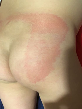
In this paper, from the set of images under study (see Fig. 1), one with good resolution and for which the size in pixels was divisible by 8, both in rows and in columns, was chosen. Furthermore, this image was a representative of a maculopapular pattern. Fig. 2 shows the chosen image, its resolution is 720×12800, and in the rest of the paper it will be called Img.
Once the color images are obtained, they are converted from the RGB to YUV color model. This model defines 3 components: 1 luminance and 2 chrominance. Therefore, now each image consists of 3 arrays of equal dimensions. And the aforementioned image (i.e., Img) has three components: Img1, Img2, and Img3. Each of these three matrices is divided into non-overlapping 8×8 matrices, and each of the blocks formed by those submatrices forms a vector of dimension 64.
Next, for the luminance matrix (i.e., the Img1 matrix) a matrix of blocks of dimension 144000×64 is formed, which we will call X1 and in which each row represents the vectors previously formed. Likewise, this process is repeated for the two chrominance matrices (i.e., Img2 and Img3), forming the X2 and X3 matrices for the Img2 and Img3 matrices respectively. So now, for each image we will have three block matrices, and to each of these matrices we apply the method of principal components with periodicity.26,27,28,29
After analyzing the decomposition of Img for each of the matrices Img1, Img2 and Img3, in order to decide the number of PCs to choose, we first analyze the growth of explained variability. In this sense, the number of PCs to take into account would be the one that exceeds a certain threshold. We worked with a threshold equal to 90%. Knowing the number of PCs, we will know the compression rate, CR. Specifically, if to compress lossless we need 64 PCs, and we compress m PCs, then the compression rate will be given by (eq:1).
Another aspect to consider is to check the quality of the compression to know if the process is efficient. To measure the quality of the compression, we will use the peak signal-to-noise ratio (PSNR) coefficient,26,29 which compares the differences between the compressed image and the original image to verify the quality. We will also calculate the mean square error (MSE) of the differences between the original and compressed images.26,29
Finally, it will be a doctor who would give the go-ahead to find out if the compressions performed meet the expected expectations. In this case, the dermatology specialists who are members of the work team will confirm that the reconstructions of the compressed medical images can be used to diagnose and classify the disease.
Results and discussions
To apply the method described in section methodology, the image under study (i.e., Img) is divided into blocks and decomposed into PCs. Fig. 3 shows the first largest eigenvalues and the explained variability by selecting those eigenvalues for the first matrix of Img (i.e., Img1) with its matrix of blocks X1. We carried out this analysis for the three matrices of Img, and built the X2 and X3 block matrices as well. These block matrices turned out to be analogous, in the sense that the first eigenvalue is very large (99.1427) compared to the second (0.5270). Furthermore, the growth of the explained variability stabilized from two principal components. Moreover, with the first two PCs, more than 99.6% of the variability shown by the matrix of the image blocks is obtained (Fig. 3B).
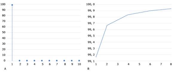
Fig. 3 Magnitude of the first eigenvalues and explained accumulated variance. A. Magnitude λ k of the first 10 eigenvalues 𝑘, 𝑘=1…10 ; B. Cumulative variability 𝐼 𝑘 explained with the first 8 eigenvalues 𝑘, 𝑘=1…8 .
PSNR and MSE of the original image versus the compressed images are then calculated, as PCs are added to the compression. Fig. 4 shows these coefficients for the selected image (i.e., Img). In addition, this figure shows that from the first principal component the PSNR is greater than 30 and that this value grows, of course, until it reaches 100, which is the value obtained by considering all the principal components. This figure also shows a very strong drop in the value of the MSE, when taking the first 10 principal components. After this value, the MSE gradually falls to 0. The two graphs shown in Fig. 4 allow selecting the number of principal components with criteria based on the quality of the compression.
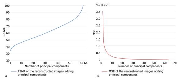
Fig. 4 PSNR and MSE of the original image versus the compressed images as PCs are added to the compression. A. PSNR of the original image versus the compressed images; B. MSE of the original image versus the compressed images.
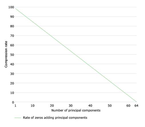
On the other hand, the compression rate (see 1) decreases linearly as more principal components are used for compression. Fig. 5 shows the evolution of the compression rate as more principal components are added.
In view of the obtained results, we decided to compress with one and two CPs. By compressing the Img image with two CPs, an explained variability of 99.6%, a PSNR of 38.2797, and a compression rate of 96.8% are obtained. While when compressing the same image with only one CP, the explained variability drops to 99.1%, the PSNR also drops to 34.2335 and the compression rate rises to 98.4%. Fig. 6 shows the result of the compressions.
When saving the compressed images in .jpg format, the size of the original image is 45060 bytes and that of the compression with two CPs is 24274 bytes, this being 53.9% of the size of the original image. Regarding the compression with one CP, the size of this is 22561 bytes, being 50.1% of the size of the original image.
Next, we verify that, effectively, when making the graphs of the first PCs, they present periodic characteristics. Fig. 7 shows the graphs of the first three PCs of X1. As can be seen, the values of the first PC are almost all the same, ranging from 0.1242 to 0.1258. So, they almost form a horizontal line. Thus, we compute the 8 median values with lag 8, generate a vector of period 8 and size 64, and substitute it into the first principal component. We do this for each of the three matrices X1, X2 and X3.
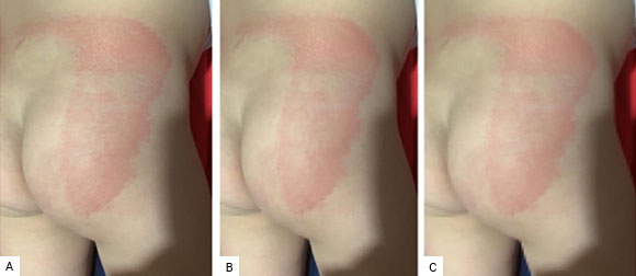
Fig. 6 Original image compressed by using one and two PCs. A. Original image: A maculopapular pattern; B. Original image compressed by using two PCs; C. Original image compressed by using one PC.
In Fig. 7B, the second PC shows a linear trend. After removing that trend, we take the residuals, recalculate the median of the values with lag 8, generate a vector of period 8 of dimension 64, and add the previously removed trend to this vector.
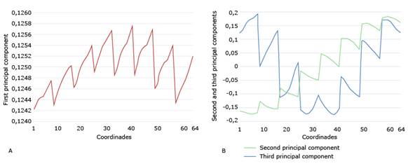
Fig. 8A shows the compression of the original image with only one periodic PC. In this case, the PSNR is 24.0421 and the compression rate is 99.8%. In this case, since the PSNR is less than 30, the compression has a low quality. This is noted because this reconstructed medical image is virtually devoid of sufficient color to show manifestations of dermatological disease.
On the other hand, the compressed image with two PCs, the first of these being the one that was replaced by periodicity, is shown in Fig. 8B. This image has a PSNR value of 38.2492 and its compression rate is 98.2%. Furthermore, the compressed image with two periodic PCs is shown in Fig. 8C. The PSNR of this image is 33.7260 and the compression rate is 99.6%.
The compressed image in .jpg format with a periodic PC has a size of 19677 bytes, which is 43.7% of the size of the original image. The image compressed with two PCs, the first PC being periodic, has a size of 21240 bytes, being 47.1% of the original image size. And, for compression with two periodic PCs, the size of this image is 20642 bytes, which is 45.8% of the original image size.
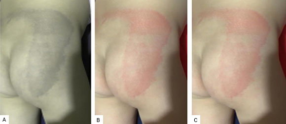
Fig. 8 Different compressions of the original image, with one and two PCs, and using the periodicity of the first PCs. A. One periodic PC; B. Two PCs, with the first periodic; C. Two PCs, with both periodic.
After explaining the principal component and periodic principal component methods applied to the medical image that represents a maculopapular pattern, Table presents a summary of the characteristics of the compressions performed.
Table Characteristics of compressed images
| Compression | Explained cumulative variability | PSNR | Compression rate (%) | Image size reduction (%) |
|---|---|---|---|---|
| One PC | 99.1 | 34.2335 | 98.4 | 49.9 |
| Two PCs | 99.6 | 38.2797 | 96.8 | 46.1 |
| One Periodic PC | - | 24.0421 | 99.8 | 56.3 |
| Two PCs, with the first periodic | - | 38.2492 | 98.2 | 52.9 |
| Two PCs, with both periodic | - | 33.7260 | 99.6 | 54.2 |
From the point of view of dermatology, the doctors that were consulted expressed that in all the photos one of the most frequent patterns in COVID-19, the maculopapular or morbilliform pattern, can be observed with very good sharpness and clarity. This pattern is clinically manifest in the patient shown in Fig. 2 and is characterized by a widespread erythmatopapular rash on the lower back. This rash extends to the right buttock in almost its entirety. In addition, in the medical images shown, both in the original and in the reconstructed ones, erythematous papules can be seen, some of the normal color of the skin, small, a few millimeters long, some of them raised and others not. Also, it is observed that these papules converge, leaving areas of healthy skin inside. All this allows to reach the diagnosis of the pathology without any difficulty, both in the original photo and in those that are compressed. As discussed in this section, the lowest quality image is the compression with one periodic principal component, but even this image conveys relevant information.
Conclusions
This paper has presented a compression method for medical images that represent dermatological manifestations in paucisymptomatic patients with COVID-19. Specifically, a representative image of the maculopapular pattern was chosen, and different types of compression were performed on it, guaranteeing the validity of the compressed images to diagnose the disease. The presented method is based on principal component analysis and on the quasi-periodicity of the first principal components, in the case of medical images of patients. Good compression ratios were achieved here, while maintaining quality and relevant features. At this time of pandemic, this is of the utmost importance in the field of medicine and even more so in the specialty of dermatology, because in this, images are a fundamental pillar in the diagnosis of diseases. Therefore, being able to work with lower-weight images without losing the characteristics of the original image allows a correct diagnosis to be made and many diseases to be classified without fear of making mistakes.
Finally, it can be concluded that, with the method presented in this paper, the authors propose the use of a robust medical-image compression technique that could be very useful in the field of dermatology.

