


 Serviços customizados
 Inglês (pdf)
 Artigo em XML
 Referências do artigo
 Enviar este artigo por email
 Citado por SciELO
  Similares em
SciELO
Similares em
SciELO 
 Permalink
1.-INTRODUCTION
Many real-life classification problems lead to situations in which the distribution of the positive and negative examples is unbalanced, because individuals of some classes appear more frequently. This is known as class imbalance and it is not uncommon to have an imbalance of several orders of magnitude. As an example, Tan et al. [1] proposed a CAD system for lung nodule classification, in which they classified 111 332 candidate structures, of which only 574 structures are actual nodules. From a machine learning point of view, this imbalanced nature of the training data represents a challenge for the learning algorithm, as it biases the outcome towards the majority class, i.e. the FPs [2].
In machine learning, several methods have been proposed to handle the class imbalance [3]. A discussion of open issues and present challenges for further development in the field of imbalanced learning can be found in [4]. Typically, to provide a balanced distribution, sampling methods are used. The sampling methods can be classified in under-sampling methods or over-sampling methods, depending on if they remove or add samples to one of the classes, respectively. The combination of under-sampling and over-sampling is referred as ensemble methods.
For a clear presentation in the rest of this work, some definitions are presented. Consider a training set S=S maj ∪ S min , where S maj and S min are the majority and minority class respectively, such that S maj ∩ S min ={∅}. The samples x i ∈ S maj and y j ∈ S min will denote individuals of the majority and minority classes, respectively. Finally, any set generated from sampling methods on S are labeled as R.
1.1.-SAMPLING METHODS FOR DATA IMBALANCE
A first group of methods resample the classes in a random fashion, either by augmenting the S min or reducing the size of S maj . The random over-sampling method augments S min replicating randomly selected examples. In this way, the class distribution balance is adjusted. On the other hand, random under-sampling works by removing randomly selected samples from S maj instead of adding samples. These two mechanisms provide a way for varying the degree of class balance in any desired way. Despite of its simplicity, each method is associated with issues that can compromise the performance of the learning algorithm [5], [6], [7].
The drawback of random under-sampling is obvious as the removal of samples from S maj can cause the classifier to miss useful information. Inversely, the over-sampling method can lead to overfitting, due to the replication of some of the samples from S min . Overfitting could make the decision rules too specific, with high accuracies on the training set, but poor performance on the testing set [5].
Condensed nearest neighbor CNN) samples S maj , eliminating random samples without significantly affecting the performance of the nearest neighbor classification, i.e. the nearest neighbor rule used to classify S maj should give almost the same result if applied to the under-sampled set R [8]. This is especially true if the elements in R are representative elements of the S maj .
Tomek links (TL) is a data cleaning technique used to remove the overlap introduced by sampling methods. A Tomek link is a pair (x i ,y j ) such that x i and y j are minimally distanced nearest neighbors. Well-defined class clusters (R) can be established removing all x i from the Tomek links until all minimally distanced nearest neighbor pairs belong to the same class. This method will lead to well-defined classification rules for improved classification performance [3].
The Near Miss methods are other data cleaning techniques for under-sampled data sets. Three variants of Near-Miss are presented in [9]. NearMiss-1 (NM1) selects the x i neighbors closest to some determined number of y j and removes them if the average distance is minimal. NearMiss-2 (NM2) works in a similar manner but considering all the y j , and taking the average distance to a determined number of the farthest y j . The third method, NearMiss-3 (NM3), selects a given number of x i , surrounding each y j . The performance of these methods could be influenced by the distribution of the x i among the y j [9].
The Synthetic Minority Oversampling Technique (SMOTE) generates synthetic examples operating in feature space [10]. S min is over-sampled by taking each y j and introducing synthetic examples along the line segments joining all of their nearest neighbors. Depending on the amount of required over-sampling, samples from the k-nearest neighbors are randomly chosen. Despite its great success in several applications, it has some drawbacks including over-generalization.
The Adaptive Synthetic (ADASYN) approach adaptively creates different amounts of synthetic data according to their distributions [11]. It uses a density distribution as a criterion to automatically decide the number of synthetic samples that need to be generated for each y j by adaptively changing the weights of different x i to compensate for the skewed distributions.
A Self-Organizing Map (SOM) aims to reduce the class imbalance by first clustering all x i samples into different cells of a Kohonen layer based on the similarities in the feature space. The subset R is generated by taking a number of examples from each cell. In this way, the size of S maj is reduced without altering the distribution in the feature space. This method was employed by Tan et al. [1] to reduce the class imbalance of the lung nodule classification problem to a factor three.
There is a third category, referred as ensemble methods, that combines over-sampling and under-sampling. Two examples of ensemble methods are SMOTE-TL and SOM-SMOTE. In SMOTE-TL, S min is oversampled with SMOTE to the size of S maj , then both classes are down-sampled to the original size of S min using TL. On the other hand, SOM-SMOTE, first down-sample S maj to a size greater than the size of S min , and then S min is oversampled to the new S maj size. As SOM-SMOTE reduces the sizes the classes as the first step, balanced data sets with less computational load can be obtained.
1.2.-CAD OF LUNG CANCER
Lung cancer has been the most common type of cancer for several decades and the second cause of death worldwide among all non-communicable diseases1. Also, its detection in initial states is considered the most effective way to improve survival of patients, in which case, the 5-year survival rate is approximately 54 %, compared to 4 % in case of detection in advanced stages [12]. These facts have led to the development of screening programs in United States of America [13,14] and Europe2. The implementation of the programs at large scale will increase the radiologist burden significantly and the computer-aided diagnosis (CAD) systems may play a significant role in reducing the reading time and thereby improving cost-effectiveness [15,16].
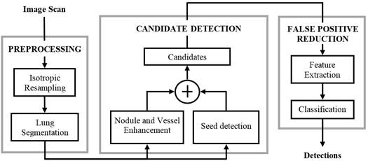
A typical CAD approach for lung cancer detection has three steps: preprocessing, candidate detection, and false positive reduction. The preprocessing is used for image standardization (spatially resampling the image to isotropic and homogeneous resolution) and lung segmentation in order to restrict the search space. The candidate detection step aims to detect nodule candidates at a very high sensitivity. As a consequence, a large imbalance between true positives (TP) and false positives (FP) is generated. Subsequently, the FP reduction step lowers the number of FPs among thecandidates and generates the final set of detected nodules. Figure 1 depicts the CAD system presented in [1], where the three steps of the procedure are shown.
1.3.-THE LUNA16 CHALLENGE
To allow the comparison of different CAD systems of lung nodules, an online framework for the evaluation was introduced in [17]. The LUng Nodule Analysis 2016 (LUNA16) Challenge has a web interface to evaluate algorithms and compare the results with other approaches. LUNA16 consists of two separate tracks: the full pipeline of a CAD system (track 1) for thoracic CT images, including the candidate nodule detection and the FP reduction; and a simplified track (track 2) covering only the FP reduction for which coordinates of candidate nodules are given. In both tracks, the data originates from the LIDC-IDRI database, consisting of a subset of 888 scans for which reference annotations from four radiologists are available [18]. This data set can be used for training and system evaluation.
In order to evaluate the systems, the Free-response Receiver Operating Characteristic (FROC) analysis is computed. TP are defined as nodules annotated by the majority of the radiologists (at least 3 out of 4 radiologists). Sensitivity is defined as the fraction of detected TP divided by the number of nodules in the LUNA16’s reference standard. In the FROC curve, sensitivity is plotted as a function of the average number of FP per scan (FPs/scan). Evaluation is performed using predefined subsets for 10-fold cross-validation, which can be downloaded from the LUNA16 website. As overall score, the average of the sensitivity at 0.125, 0.25, 0.5,1, 2, 4, and 8 FPs per scan, over all folds, is used. Also, the 95% confidence interval using bootstrapping with 1000 bootstraps is calculated. For each bootstrap, a new set of candidates are constructed using (scan-level) sampling with replacement. A Python evaluation script is available for download on the LUNA16 website and the results can be viewed by all participants.
1.4.-CAD SYSTEMS AND DATA BALANCE
Classifiers with balanced data sets tend to perform better, in particular in terms of increasing sensitivity at low FP rates [10]. As mentioned, CAD systems typically face this problem as well. Despite this, few data balance studies for CAD of lung nodules have been reported. Table 1 shows an overview of previous work in classical CAD system development.
Table 1 Data sets and data balance methods reported in classical CAD systems for lung nodule detection.
| Number of scans | Data balance method | Number of scans | Data balance method | ||
|---|---|---|---|---|---|
| Tan et al. [1] | 450 | SOM | Han et al. [19] | 1012 | - |
| Abbas [19] | 220 | - | Madgy et al. [21] | 80 | - |
| Nithila and Kumar. [20] | 106 | - | Orozco et al. [23] | 45 | - |
| Cirujeda et al. [21] | 95 | - | Badura and Pietka [25] | 23 | - |
| Jacobs et al. [22] | 888 | - | Sun et al [27] | 360 | SMOTE |
| Firmino et al. [23] | 420 | - | Keshani et al. [29] | 50 | - |
| Demir and Çamurcu. [24] | 95 | - | Shiju et al. [31] | 108 | SMOTE |
| Gong et al. [25] | 189 | SMOTE | Jingchen et al. [33] | 1010 | SMOTE |
| Demir and Çamurcu. [26] | 200 | - | Makaju et al. [35] | 1018 | - |
| Baboo and Iyyapparaj [27] | 1028 | - | Cao et al. [37] | 1012 | MKFSOS |
| Sui et al. [28] | 120 | RU-SMOTE | Mehre et al. [39] | 97 | SMOTE |
As can be seen, most of the reviewed works on classical CAD systems for lung nodules do not report the use of any data balancing methods. Few authors mention data balancing, but did not examine the impact with respect to unbalanced data. To the best of the authors knowledge, only Sui et al. [38] described the impact of data balancing for CAD of lung nodules. In their experiments, 500 candidate nodules from 120 patients, with a class imbalance of 1/6, were classified based on eight features using several techniques to deal with class imbalance. They found that considerable improvement can be obtained by alleviating the data imbalance -the best results obtained using a combination of under- and oversampling together with a biased SVM approach.
The purpose of this paper is to compare the performance of different data balancing techniques applied to the classification of a highly imbalanced biomedical dataset and their impact on nodule classification tasks. With respect to previous work, the presented experiments are based on a larger data set, have higher feature dimensionality, include more data balancing techniques and evaluate sensitivities at both low and high FP rates.
2.-MATERIAL AND METHODS
2.1.-THE ETROCAD SYSTEM
A modification of the system proposed in [1], referred in the rest of this paper as ETROCAD is used to evaluate the effect of data balancing techniques on the performance of a CAD system. The ETROCAD system is modified in terms of using a Support Vector Machine (SVM) with radial basis function kernel. SVMs are well-established classifiers, proven to be useful in many cancer classification tasks [1,28-40].
The 888 scans from the LUNA16 framework were processed by the first two steps of the approach in Figure 1 (preprocessing and candidate selection) to extract all the candidates. A feature vector is built by features calculated for each candidate. Table 2 shows a short summary of the used features [1].
Table 2 Description of features used in ETROCAD
| Feature | Notes |
|---|---|
| Volume | Equivalent to the number of voxels |
| Min_diam = min(dimi) | Dimi=minimum diameter corresponding to the principal axis i of the minimum volume-enclosing ellipsoid |
| Max_diam = max(dimi) | |
| Compactness1 | Ratio between volume and product of all dimi |
| Compactness2 | Ratio between volume and dimi 3 |
| Elongation factor | Max_dim/min_dim |
| Bounding ellipsoid feature | 1 for 3D ellipsoid, 0 for 2D ellipsoid |
| Distance to lung wall | From nodule candidate centroid to lung wall |
| Distance to the center of the slice | From candidate centroid to the center of the slice on which centroid is located |
| Average of Luu and Lvv | On segmented voxels, and spherical kernels of radius 1 and 3 pixels at scales 1 and 2. Luu and Lvv features over a gauge coordinate system [1]. |
| Average of nodule filter values | On segmented voxels, and spherical kernels of radius 1 and 3 |
| Average of vessel filter values | On segmented voxels, and spherical kernels of radius 1 and 3 |
| Average of divergence values | On segmented voxels, and spherical kernels of radius 1 and 3 |
| Grey-value features | Mean, median, maximum, minimum and standard deviation on segmented voxels, and spherical kernels of radius 1 and 3 |
2.2.-BALANCING THE DATA
The SOM-based method was implemented using a SOM Toolbox for Matlab3.In this case, the TP/FP ratio was 1/3 to be consistent with the original system [1]. The rest of data balancing methods and classification were implemented in Python 2.7, using the Imbalanced-learn [41] and the Scikit-learn4 modules respectively. Scikit-learn provides easy-to-use tools for data mining and data analysis. Table 3summarizes the methods implemented in Scikit-learn that were used on the lung nodule data provided by the ETROCAD system. In all the cases, the goal was to get a well-balanced dataset with a final TP/FP ratio approximating 1.The remaining parameters of the methods were set to recommended default values.
2.3.-DATA SET PROCESSING AND EVALUATION
To evaluate the different methods, the feature vectors provided by ETROCAD were balanced by each of the data balancing methods from Table 3. The result was then used to train the ETROCAD’s classifier.
The performance of each method was evaluated using the methodology provided by the LUNA16 framework (track 1). The 10-fold cross-validation was run as described in LUNA16 procedure, and then the FROC curve and the score were calculated (average of sensitivities at 0.125, 0.25, 0.5,1, 2, 4, and 8 FPs per scan).To be able to compare the methods, the evaluation script from LUNA16 was modified to extract all the FROC curves from bootstrapping; and all the scores for each one were calculated.
Table 3 Sampling methods and default values for methodsused in imbalance learning.
| Method | Parameter name | Default value |
|---|---|---|
| RUS | No parameters | - |
| TL | No parameters | - |
| NM-3 | Number of neighbors to be considered | 3 |
| CNN | No parameters | - |
| ROS | No parameters | - |
| SOM | FP-TP ratio | 3 |
| SMOTE | Number of nearest neighbors to construct the synthetic samples | 5 |
| ADASYN | Number of nearest neighbors to construct the synthetic samples | 5 |
| SMOTE-TL | Number of nearest neighbors to construct the synthetic samples | 5 |
| SOM-SMOTE | FP-TP ratio | 3 |
| Number of nearest neighbors to construct the synthetic samples | 5 |
Kruskal-Wallis test is used to find if there are differences at the 1 % of significance level. If differences are found, a multiple comparison is done using the Bonferroni method. Kruskal-Wallis test and multiple comparisons are done using kruskalwallis and multcompare functions respectively from Matlab’s Statistical and Machine Learning Toolbox.
3.-RESULTS
At the output of the candidate detection phase, ETROCAD detected 435 303 structures (candidates) in 888 scans, of which 1186 correspond to actual nodules according to the ground truth annotations provided. As such, the initial imbalance ratio was approximately 367. Figure 2 shows the graphical output obtained with LUNA16 script for SMOTE. The solid line represents the FROC curve for the system with the balance method and dashed lines mark the limits for a 95 % confidence interval of the bootstrapping procedure.

Figure 2 LUNA16 script output for SMOTE. Solid line: FROC curve for the 10-fold cross-validation, dashed lines: limits for the 95 % confidence interval from bootstrapping. Mean curve is overlapped with the solid line.
From the modified LUNA16 script, 1000 FROC curves were extracted from the bootstrapping procedure for each balancing method. Table 4 shows the mean scores and standard deviations for all sets of curves. Differences at 1 % of significance level were found among the populations using the Kruskal-Wallis test (p-value = 0).
Table 4 Mean scores and standard deviations for all curves from bootstrapping
| No Balance | SOM | CNN | RUS | NM-3 | TL | ROS | ADASYN | SMOTE | SMOTE-TL | SOM-SMOTE | |
|---|---|---|---|---|---|---|---|---|---|---|---|
| Mean score | 0.748 | 0.704 | 0.55 | 0.655 | 0.422 | 0.749 | 0.743 | 0.730 | 0.760 | 0.760 | 0.745 |
| Standard deviation | 0.018 | 0.023 | 0.018 | 0.019 | 0.017 | 0.018 | 0.020 | 0.019 | 0.019 | 0.018 | 0.019 |
Figure 3 shows the graphical output from the Matlab’s multcompare function. This graph shows the estimates and a pair wise comparison in which two groups are significantly different if their intervals (horizontal lines) are disjoint. In this way, only SOM-SMOTE and TL, have no significant differences with NoBalance. The best overall performance was obtained using SMOTE and SMOTE-TL methods.
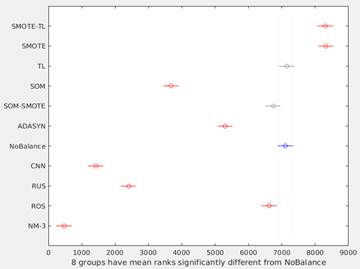
Figure 3 Differences among methods using multiple comparison test. Because Kruskal-Wallis test was used, horizontal axis corresponds to the ranks of the median for each method. SOM-SMOTE and TL (gray lines) have no significant differences respect to NoBalance (blue line).
A more detailed analysis of the sensitivities at different FP rates is shown in Table 5, along with final average score for each method. For the lowest FP rate (0.125FP/scan), all evaluated methods except for TL have scores below the system with no data balancing. All over-sampling and ensemble methods achieve higher overall scores than the under-sample ones.
Table 5 Sensitivities at selected FP per scan and scores as defined in LUNA16 Challenge
| FP/Scan | No Balance | SOM | RUS | CNN | NM-3 | TL | ROS | ADASYN | SMOTE | SMOTE-TL | SOM-SMOTE |
|---|---|---|---|---|---|---|---|---|---|---|---|
| 0.125 | 0.578 | 0.245 | 0.344 | 0.384 | 0.294 | 0.581 | 0.486 | 0.453 | 0.540 | 0.538 | 0.515 |
| 0.250 | 0.663 | 0.509 | 0.488 | 0.431 | 0.332 | 0.663 | 0.618 | 0.590 | 0.650 | 0.652 | 0.628 |
| 0.500 | 0.718 | 0.647 | 0.606 | 0.485 | 0.368 | 0.718 | 0.724 | 0.707 | 0.740 | 0.738 | 0.728 |
| 1.000 | 0.773 | 0.750 | 0.696 | 0.535 | 0.420 | 0.775 | 0.783 | 0.780 | 0.792 | 0.793 | 0.778 |
| 2.000 | 0.805 | 0.810 | 0.772 | 0.594 | 0.458 | 0.810 | 0.834 | 0.824 | 0.839 | 0.838 | 0.824 |
| 4.000 | 0.837 | 0.854 | 0.822 | 0.672 | 0.513 | 0.836 | 0.864 | 0.862 | 0.868 | 0.864 | 0.862 |
| 8.000 | 0.860 | 0.886 | 0.858 | 0.755 | 0.581 | 0.860 | 0.885 | 0.882 | 0.890 | 0.889 | 0.891 |
| Score | 0.748 | 0.672 | 0.655 | 0.551 | 0.424 | 0.749 | 0.742 | 0.728 | 0.760 | 0.759 | 0.747 |
Figure 4 shows the FROC curves for all methods. As can be seen, curves for NM3, CNN and RUS are always below NoBalance. SOM goes over NoBalance only at FP rates higher than 2FP/Scan. The sensitivity values for TL are almost the same than NoBalance. On the other hand, the rest of the methods but ADASYN go higher than NoBalance for FP rates higher than 0.5 FP/Scan.
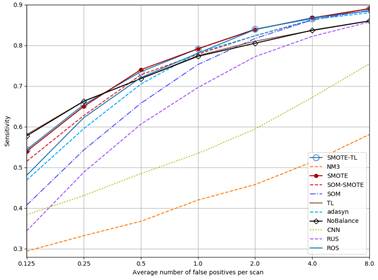
Figure 4 FROC curves for each method. SMOTE and SMOTE-TL as well as TL and NoBalance are overlapped.
To highlight the impact of data balancing, Table 6 shows a summary of the results obtained at 4 FP/scan, a value commonly used in a clinical setting. For the best method, data balancing resulted in 36 additional nodules correctly classified.
Table 6 Summary for the selected ETROCAD versions. The first row corresponds to the system with no balance method; the other rows are sorted in ascendant order according to sensitivity (Sens). dTP, dTN, dFP and dFN are the detection differences respect to the no balanced system. Negative numbers represent less detections than NoBalance. All values are reported at 4 FP/scan
| Method | TP | TN | FP | FN | dTP | dTN | dFP | dFN | Sens (%) | Spec (%) | Acc (%) |
|---|---|---|---|---|---|---|---|---|---|---|---|
| NoBalance | 992 | 80025 | 3434 | 194 | - | - | - | - | 83.73 | 5.35 | 1.40 |
| NM3 | 608 | 80774 | 3547 | 578 | -384 | 749 | 113 | 384 | 51.35 | 14.01 | 1.39 |
| CNN | 796 | 80227 | 3538 | 390 | -196 | 202 | 104 | 196 | 67.20 | 9.93 | 1.40 |
| RUS | 974 | 79685 | 3522 | 212 | -18 | -340 | 88 | 18 | 82.21 | 5.68 | 1.41 |
| TL | 991 | 79882 | 3545 | 195 | -1 | -143 | 111 | 1 | 83.64 | 5.21 | 1.40 |
| SOMSMOTE | 1022 | 74648 | 3550 | 164 | 30 | -5377 | 116 | -30 | 86.17 | 4.42 | 1.49 |
| SOM | 1023 | 78623 | 3551 | 163 | 31 | -1402 | 117 | -31 | 86.26 | 4.39 | 1.42 |
| ADASYN | 1023 | 79479 | 3487 | 163 | 31 | -546 | 53 | -31 | 86.34 | 4.47 | 1.41 |
| SMOTETL | 1026 | 79505 | 3500 | 160 | 34 | -520 | 66 | -34 | 86.59 | 4.37 | 1.41 |
| ROS | 1028 | 79495 | 3520 | 158 | 36 | -530 | 86 | -36 | 86.76 | 4.30 | 1.41 |
| SMOTE | 1028 | 79492 | 3533 | 158 | 36 | -533 | 99 | -36 | 86.76 | 4.28 | 1.41 |
4.-DISCUSSION
Under sampling methods were found to perform badly in the experiments. Both, RUS and NM3 remove samples without considering whether they are “good examples” of FP. This may have hampered the performance of the system, which is confirmed by the reduced score of both methods. On the other hand, as TL tries to get a well-defined set for training by removing boundary or noisy samples, it is expected to perform better than other methods. For the cases of SMOTE and SMOTE-TL, they were found significant better than the rest of the methods, as can be seen from the Table 4 and Figure 3, although the relative difference in the score is only 0.1 % with respect to no balancing.
When considering the LUNA16 score, differences between the methods are relatively small in terms of average sensitivity, Table 6). This can be attributed to averaging of sensitivities at different FP rates, and the high number of candidate structures. At 4 FP/scan, and when considering the absolute number of detections, the difference is more apparent.
The performance of the employed CAD system is comparable to the state of the art. Most studies report sensitivities at high FP rates. Achieving high sensitivity at low FP rates is technically challenging, but more suitable for clinical use, which is why it was included in current study. Mehre et al. [39] report sensitivities of 92.91 % at 3 FP/scan. Although this value is higher than the values shown at Table 4, their performance at lower FP rates is worse. To be able to get the values at lower FP rates, the sensitivities at 0.125, 0.25, 0.5, 1, 2, 4, 8 FP/scans from the FROC curve in [39] were estimated using WebPlotDigitizer5. The estimated sensitivities were 0.2, 0.34, 0.53, 0.73, 0.87, 0.96 and 0.98; yielding a LUNA16 score of 0.66, which is lower than the best scores reported in Table 5.
The improvement for lung nodule classification when using data balancing reported by Sui et al. [38], was larger with respect to the results obtained in this study. Detailed comparison is however difficult, as differences could be due to the different dataset, the limited amount of scans used in latter study (120 scans) and the low-dimensional feature space.
The impact of proper data balancing can be seen when considering the results of the LUNA16 Challenge (https://luna16.grand-challenge.org/results/). In December of 2017, the ETROCAD system using SOM, ranked 15thout of 18 participants in track 1 of the competition (competition metric: 0.672). The same system, i.e. using the same candidate detector, feature extraction and classification; but using SMOTE or SMOTE-TL as a data balancing method instead of SOM, would achieve a 13th place (competition metric: 0.759) and become the highest ranking system based on handcrafted features (all the systems with higher scores use deep-learning techniques). One should consider the improvement was obtained without adding any additional data or priors to the classification problem.
5.-CONCLUSIONS
In this work, the influence of data balancing techniques on a lung CAD system was evaluated using a web-based framework. Data balancing techniques can be useful to improve the efficiency or boost the performance of classification. The use of data augmentation is always advisable since, although changes in the sensitivity may seem marginal for a big training set, an improvement in the quality of the detection in absolute values can be seen. These methods can have a significant impact on the training process of the SVM, making the generation of classification rules easier. For the application of lung nodule classification, SMOTE and SMOTE-TL were found to perform best, leading to a gain in sensitivity, in particular at lower FP rates. Although, balancing the data can improve the performance of the classification, this is only one factor to take into account in machine learning.

