Artículo original

Assessing different models to estimate photovoltaic monocrystalline modules operating temperature using weather data

Evaluación de diferentes modelos para estimar la temperatura de operación de módulos fotovoltaicos monocristalinos usando datos climatológicos

0000-0001-5217-318XLiomnis Osorio Laurencio^{I  *}  , 0000-0002-5098-5675Yoalbys Retirado-Mediaceja^I  , 0000-0002-2289-8160José Emilio Camejo Cuán^II  , 0000-0003-2575-2690Roger Proenza Yero^II  , 0000-0001-6740-4753Adrián Romeu Ramos^II  , 0000-0002-1984-0822Eliannet Varga Estupiñan^III 

^I Universidad de Moa, Dr. Antonio Núñez Jiménez (UMoa). Holguín, Cuba

^II Centro de Investigaciones de Energía Solar (CIES). Santiago de Cuba, Cuba

^III UEB Fuel Oíl Lidio Ramón Pérez. Moa, Holguín, Cuba

ABSTRACT

The efficiency of photovoltaic modules depends on the operating temperature of the cells. Currently it is difficult to choose a suitable model to estimate the temperature of the modules, due to the variety of proposed models. In this research, ten temperature estimation models of the modules were evaluated, based on three input variables: ambient temperature, irradiance and wind speed. For the modeling, in situ measurements were used, recorded for six months, by the 7.5 kWp monocrystalline silicon photovoltaic system and a climatological station of the Solar Energy Research Center of Santiago de Cuba. King et al (2004) was the model with the best accuracy criteria, with squared error, mean absolute error and coefficient of determination equal to 3.482 ºC, 2.698 ºC and 0.912, respectively. Finally, the effect of the operating temperature of the modules on the efficiency was simulated, obtaining useful information for future projects of photovoltaic systems in Cuba.

Key words: cell efficiency; mathematical modeling; module temperature estimation; weather data of Cuba

RESUMEN

La eficiencia de los módulos fotovoltaicos depende de la temperatura de operación de las celdas. Actualmente es difícil escoger un modelo idóneo para estimar la temperatura de los módulos, debido a la variedad de modelos propuestos. En esta investigación se evaluaron diez modelos de estimación de temperatura de los módulos, a partir de tres variables de entrada: temperatura ambiente, irrandiancia y velocidad del viento. Para las modelaciones se usaron mediciones in situ, registradas durante seis meses, por el sistema fotovoltaico de silicio monocristalino de 7,5 kWp y una estación climatológica del Centro de Investigaciones de Energía Solar de Santiago de Cuba. El modelo King et al. (2004) presentó los mejores criterios de precisión, con error cuadrático, error medio absoluto y coeficiente de determinación igual a 3.482 ºC, 2.698 ºC y 0.912 respectivamente. Finalmente, se simuló el efecto de la temperatura de operación de los módulos sobre la eficiencia, obteniéndose informaciones de utilidad para futuros proyectos de sistemas fotovoltaicos en Cuba.

Palabras-clave: eficiencia de las celdas; estimación de temperatura de la celda; modelación matemática; datos del clima de Cuba

Introduction

The photovoltaic solar energy (PV) has experienced an accelerated increase compared to the previous year, despite the global economic crisis caused by Covid-19 ^[1]. Reports published by International Energy Agency and National Renewable Energy Laboratory’s in 2022 show that in first nine months of 2021 the capacity of 171 GW of photovoltaic systems installed globally throughout the world was reached, while for 2022 and 2023 it’s expected to reach 209 GW and 231 GW respectively ^[1], ^[2]. According to statistics report published by International Renewable Energy Agency in 2021, Cuba ended that year with 163 MW of installed capacity of photovotlaic systems ^[3]. The Ministry of Energy and Mines has the plan of reaching 24% penetration with renewable sources by 2030 ^[4].

For this reason, studies about the renewable energy sources have increased, such is the case of Díaz (2018), Gutiérrez et al., (2020); Gutiérrez et al., (2021a); Gutiérrez et al., (2021b), all the results have contributed to improving the efficiency of PV systems in the country ^[4], ^[5], ^[6], ^[7]. Even Korkiakoski (2021) and Alberto et al., (2021) studied the possibility of generating 100% energy from renewable sources by 2030, the Isla de la Juventud was taken as case study; demonstrating that’s possible to achieve it ^[8], ^[9]. The weather conditions in Cuba are very good for the development of solar energy, however, it’s a tropical island where the ambient temperature is higher than other regions of the world. Temperature is the climate variable that most affects the efficiency of the PV module, after irradiance ^[10]. Conventional photovoltaic cells are made of semiconductor material that produces electrical energy from the solar radiation that reaches it’s surface. In the process of converting from one type of energy to another, there are losses associated with various factors such as: production technology, shading, module temperature, angular losses, inverter losses, and cable losses. These parameters cause losses of 10-20%, being those that most affect the efficiency of photovoltaic conversion ^[11], ^[12].

Many investigations have correlated the efficiency with the operating temperature, the PV cell only converts a small amount of the irradiance it receives into electrical energy, the rest is dissipated as heat ^[13]. The electrical efficiency ηc is expressed as a function of the cell temperature Tc through the linear relationship shown in equation (1), ^[14]. This correlation has been widely accepted and for this reason it appears in experimental investigations for different environmental conditions ^[15], ^[16].

(1)

Where n _STC (%) and β _STC (%/°C) are the electrical efficiency and temperature coefficient of the cell, respectively. Tc (°C) and T _STC (°C) are the cell operating temperature and the reference temperature, respectively. The n _STC , β _STC and T _STC parameters are always provided at the PV module technical datasheet. The operating temperature Tc is a variable that is not commonly measured, but can be calculated by applying mathematical models that correlate some weather variables. Current models mainly correlate three climate variables: ambient temperature, irradiance and wind speed. These models are classified into three groups: constant temperature models, physical models and statistical models ^[17]. Some of these models do not use wind speed, while others do, the latter being the ones that have shown better accuracy in most of the studied cases ^[18].

Literature review: PV cell operating temperature estimate models

Constant temperature models use a constant value of the photovoltaic cells operating temperature to estimate the energy delivered for specific conditions of PV system. This type of model has the advantage that it can be used quickly to predict the performance of PV systems, since manufacturers always include the necessary parameters at the technical datasheet. The most used are the Standard Measurement Conditions (STC) and the Nominal Operating Cell Temperature (NOCT) ^[17], ^[19]. STC are specific laboratory conditions, they are defined as: irradiance G=1000 W/m², PV cell temperature Tc=25 ºC and air mass AM=1.5 G ^[10], ^[20]. However, STC can be very different from the operating conditions of PV modules in a real environment in many places around the world. As alternative to the STC, Duffie & Beckman (2013) propose a model for NOCT conditions, defined by: G=800 W/m², Tc=20 ºC and v=1 m/s ^[19], ^[21], ^[22]. These two models have the disadvantage that the proposed environmental conditions rarely coincide with the actual operating conditions of the PV systems.

Physical models have been established to calculate the operating temperature of modules dynamically, studies by Lawrence Kamuyu et al. (2018), Nguyen et al. (2021) and Sredenšek et al. (2021) are current evidence of these research topics, each one models Tc according to it's PV technology and it's geographical installation site, respectively ^[18], ^[23], ^[24]. In addition to irradiance and ambient temperature, some models also consider wind speed King et al. (2004), Faiman et al. (2008) and Koel et al. (2011) ^[25], ^[26], ^[27]; while others do not consider it, such as Akhsassi et al.^[28]; but all agree that irradiance is the main cause that causes an increase in temperature of the PV cell. Statistical models can be subdivided into two groups: Artificial Intelligence (AI) methods and linear models. Studies that include AI to predict Tc consist of neural networks, soft computing, and adaptive neuro fuzzy inference system ^[29], ^[30], ^[31], ^[32].

These methods have the advantage of being very versatile, due to their ability to process complex trends; but as they are black box models where do not explicitly it show the relationship between the model variables. Linear statistical models are much simpler, some of the most applied in published research are Risser & Fuentes (1983) and Muzathik (2014) ^[33], ^[34]. These models correlate the module temperature (Tc) with the three main variables (G, Ta, v) in situ measured, but could be inaccurate when applied to any other site, for this reason these models need to be verified. The aforementioned studies predict the Tc from the radiation that falls on the surface of the PV cells and other measured climate variables, however, a general model that can satisfy all PV technologies has not been established. For example, Zouine et al. (2021) analyzes 48 combinations of models of the thermal and electrical behavior of PV cells of crystalline technologies, showing the diversity and relevance of this type of research ^[16].

Research aim

This research analyzes different established mathematical models, the aim is determinate the model that best correlation with Tc measurements of monocrystalline silicon PV modules, installed at the Solar Energy Research Center (CIES spanish acronym) in Santiago de Cuba. For the assessment, ten models widely referenced and recommended by the scientific community have been chosen. The variables that correlate are: ambient temperature (Ta), irradiance (G) and wind speed (v).

Also it's calculates the variation of the PV efficiency as a consequence of the behavior of the local climate variables, the results are useful to improve the reliability of the sizing of the PV systems for future projects to be developed in Cuba.

Materials and methods

Geolocation of PV system and instrumentation used in data monitoring

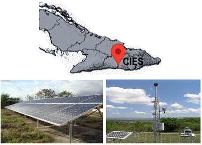
The climate data were measured at the CIES in Santiago de Cuba, a province located south of eastern Cuba. Specifically, it’s located at the geographic coordinates 20° 00′ 14″ N and 75° 46′ 10″ W, at 90.40 meters above sea level. Figure 1, shows the geolocation, the PV system and the weather station.

Fig. 1 Geographic location of PV system and the weather station of CIES in Santiago de Cuba ^[35]  

The setup of the photovoltaic generator installed in the CIES is presented in table 1, consists of 30 modules installed on the ground, grouped by 3 strings of 10 modules.

Table 1 Setup of PV system 

Type of structure	Mounted on an aluminum base, with wind circulation.
Tilt angle	15°
Azimuth angle	0°
PV power	7.5 kW

The electrical parameters of the PV module are presented in table 2, its permissible operating temperature is -40 ºC to 80 ºC, these parameters are available in the technical datasheet.

Table 2 Electrical parameters of HELIENE215MA PV module ^[36]  

Parameter	STC	NOCT
Peak Power Watts (Pmax)	250 W	183 W
Open Circuit Voltage (Voc)	37.40 V	34.5 V
Maximum Power Voltage (Vmpp)	30.3 V	27.7 V
Short-Circuit Current (Isc)	8.72 A	7.25 A
Maximum Power Currennt (Impp)	8.22 A	6.7 A
Coefficient Temperature Voc (β)	-0.34 %/°C	-
NOCT	-	45 ºC
Technology type	Monocrystalline
Efficiency	15.03 %
Cells	60 series connected cells

The meteorological parameters including irradiance and ambient temperature were measured by sensors installed next to the PV system, while wind speed was measured by a weather station placed about the 10 meters above it. The module temperature sensor was adhered to the backside of a module, ensuring good contact. The technical details of sensors and the weather station are presented in table 3.

Table 3 Technical features of the measurement instruments 

Components	Parameters	Accuracy	Model
Module’s temperature sensor	Tc (°C)	±0.8 °C (in the range -20°C to 100°C)	PT1000
Weather Station	Ta (°C)	±0.8 °C (in the range -40°C to 100°C)	METEODATA 3016 C
	G (W/m2)	±5 % (average over a year)
	v (m/s)	0.3 m/s

The data measured includes the period from September 20 (2018) to March 31 (2019), with 10-minute sampling intervals, for a total of 27,648 measurements.

Assessed Tc estimation models

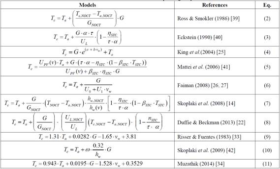
The table 4, shows 10 assessed models for the correlation of in situ measurements, including physical models, equations 2, 3, 4, 5, 6, 7, 8, and statistical models, equations 9, 10, 11. The considered models are widely known and applied in many study cases from various countries ^[24], ^[37], ^[38]. A few of them are the mathematical support of professional software, i.e. RETScreen, equation (2), PVsyst, equation (6) and System Advisor Model (SAM), equation (7), which are useful for the sizing and simulation of PV systems ^[15].

The STC and NOCT constant temperature models are not considered because it’s interesting to know the thermal performance of the modules for variable meteorological conditions. Note that equations 2, 3, 8 don’t use the wind for modeling.

Table 4 Models to estimate the module operating temperature. ^[14] , ^[22] , ^[25] , ^[26] , ^[27] , ^[33] , ^[34] , ^[39] , ^[40] , ^[41] , ^[42]  

Where

T C	the temperature of the PV cell (°C)
Ta	the ambient temperature (°C)
T c,NOCT	nominal operating temperature, depending on the manufacturing material it has a value of 44 °C to 46 °C
T a,NOCT	is ambient temperature for NOCT conditions, it has constant value of 20 °C
G NOCT	the irradiance for NOCT conditions, it has a constant value of G=800 W/m^2
G	the irradiance received at the receptor plane (W/m^2)
η STC	the module efficiency for STC conditions
τ·α	the product of transmittance-absorbance, has a constant value of 0.9 ^[14] , ^[40]
U PV	the heat exchange coefficient at the surface of the module ^[40] , ^[41]
β STC	the coefficient of variation of voltage with temperature (%/°C)
T STC	the module operating temperature for STC conditions
h W	the wind convection coefficient (W·m^-2·°C^-1)
h W,NOCT	the convection coefficient for the wind in NOCT conditions (W·m^-2·°C^-1)
v W	the wind speed measured near the module (m/s)

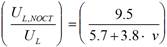
In equation (3), U _L is the heat loss coefficient, a parameter that is calculated for each module by equation (12), ^[40]:

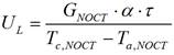(12)

In equation (4), the coefficients a and b have been calculated, obtaining a=-3.473 and b=-0.0594, the main advantage is that it does not distinguish between different PV technologies ^[10], ^[43].

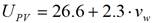
In equation (5), the parameter τ·α=0.81 while U _PV is the heat exchange coefficient, it’s a linear function with the wind speed, it has two forms of parameterization represented by equations (13) and (14), to this equations are called as Mattei1 and Mattei2, respectively ^[41]:

(13)

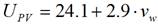(14)

In equation (6), for monocrystalline silicon technology, the constants U ₀ =30.02 and U ₁ =6.28 are used ^[27].

In equation (7) and (10), the parameter h _W is the wind convection coefficient, it’s calculated by equation (15), ^[14].

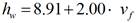(15)

Where

v f	is the wind speed measured at 10 meters above the ground (m/s) ^[10].

In equation (8), the heat exchange coefficient is approximated by equation (16), ^[38].

(16)

In equation (10), the ω parameter is a mounting coefficient defined as the ratio between the Ross parameter for the mounting geometry and the Ross parameter for free-standing modules. It takes different values: 1 for free-standing, 1.2 for flat roof, 1.8 for sloped roof (well cooled) and 2.4 for facade integrated ^[10], ^[43]. By the setup of PV system of CIES at this study ω =1 is considered.

Statistical analysis for model assessment

In order to assessment the models, the coefficient of determination (R²), the root mean squared error (RMSE) and the mean absolute error (MAE) are calculated by equations 17, 18, 19, respectively ^[32], ^[38]. These statistical indicators help to determine the difference between the temperature simulated (Tc_sim) and the temperature measured (Tc_meas).

(17)

(18)

(19)

Where

n	total number of measurements
i	index of the iteration loop
Tc_sim	simulated temperature
	simulated mean temperature
Tc_meas	measured temperature
	mean measured temperature.

Results and discussion

The eastern region of Cuba, where the CIES of Santiago de Cuba is located, is characterized by high air temperatures throughout the year. On the left side of figure 2, it shows the histogram of the Ta measured, wich easily overcomes 30 °C; on the right side, it shows the histogram of Tc measured, which easily exceeds the reference values established on the technical datasheet.

Fig. 2 Data distribution observed for Ta and Tc 

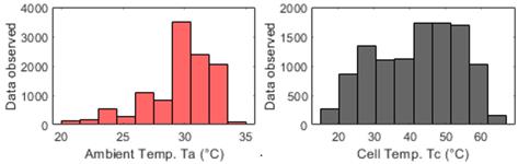
A brief statistical summary of the climate variables is presented in table 5, the data were filtered to analyze only the measurements with the condition G > 0 W/m². The filtered data removes also the night time measurements, that is, only registered measurements during daylight hours, between 6:00 to 18:00 hours were used.

Table 5 Statistical summary of the climate variables measured at CIES 

Variable	Minimum	Mean	Maximum
Irradiance (G)	1 W/m^2	513.96 W/m^2	1247.00 W/m^2
Wind speed (v w )	0.08 m/s	2.50 m/s	8.49 m/s
Ambient temperature (Ta)	20.00 °C	29.39 °C	35.00 °C
Cell temperature (Tc)	17.00 °C	41.98 °C	67.00 °C

Figure 3 and the summary of table 5, confirm that the weather conditions in Cuba, and in particular in Santiago de Cuba, are more higher than the STC conditions provided by the manufacturers technical datasheet of PV modules, in which the mean of Tc exceeds of reference (T=25 °C). Likewise, the maximum irradiance values exceed the reference value defined in technical datasheets. Hence the importance of applying the models to effectively predict Tc.

Analysis of the correlation of assessed models

The models in table 4, were correlated with the in situ measurements of Tc of the HELIENE215MA modules, applying equations 17, 18, 19 the statistical coefficients shown in table 6, were obtained. The best and worst correlation models are marked in bold.

Table 6 Statistical coefficients of the models 

Models	R^2	RMSE (°C)	MAE (°C)
Ross & Smokler (1986)	0.890	3.897	4.114
Eckstein (1990)	0.894	3.835	3.012
King et al. (2004)	0.912	3.482	2.698
Mattei1 (2006)	0.915	3.425	3.830
Mattei2 (2006)	0.913	3.468	3.659
Faiman (2008)	0.898	3.758	3.651
Skoplaki et al. (2008)	0.894	3.834	3.497
Duffie & Beckman (2013)	0.803	5.216	5.817
Risser & Fuentes (1983)	0.896	3.792	10.738
Skoplaki et al. (2009)	0.893	3.846	3.368
Muzathik (2014)	0.881	4.060	8.091

According to the accuracy criterion of the coefficient of determination R², the models with the best correlation are King et al. (2004) , the two variants Mattei (2006) and Skoplaki et al. (2009) with R² > 91%; to a lesser extent are Ross & Smokler (1986), Eckstein (1990), Faiman (2008), Skoplaki et al. (2008) and Risser & Fuentes (1983), with R² > 89%. The Duffie & Beckman (2013) model presented the worst correlation, with R² < 82%.

The Ross & Smokler (1986) model does not use the wind, however, it has a better R² coefficient than Duffie & Beckman (2013) model. The Eckstein (1990) model has a relationship with Tc that is practically the same as the Skoplaki et al. (2008), so similar R² and RMSE results were obtained for both. All the models presented a high R² correlation, which implies that any of these models could be used effectively for the estimation of Tc, but the Mattei1 (2006), Mattei2 (2006) and King et al. (2004) had very similar R² and RMSE coefficients, so any of these three could be chosen to predict Tc. In order to decide which is the best correlationed model, the MAE coefficient was taken into account as the main accuracy criterion. Figure 3, shows a scatter plot with the relationship between RMSE and MAE coefficients, which help to make a final decision.

Fig. 3 Scatter plot of the MAE vs RMSE coefficients 

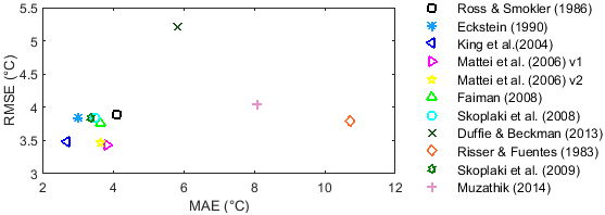
The figure 4, shows that the King et al. (2004), Mattei1 (2006) and Mattei2 (2006) models present a very small variation in terms of RMSE, but the King et al. (2004) is the model with better MAE accuracy, therefore, we considered that is the best choice to estimate Tc. For this reason, it’s recommended to use in sizing and economic feasibility studies for future photovoltaic system projects to be installed in the region.

Estimation of PV efficiency

To estimate the PV conversion efficiency of each model, the Tc values were substituted in equation 1. Figure 4, shows the linear correlation of the PV conversion efficiency with respect to Tc calculated from the model King et al. (2004). Note that the increase in temperatures has a decreasing effect on the efficiency of the PV modules, the points indicated in graph show that the efficiency decreased 1.9% for the time measured.

Fig. 4 Linear plot of Tc vs ηc, with the equation showed in graph 

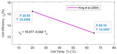
The worst model Risser & Fuentes (1983) returns maximum values of Tc=77.12 °C with MAE=10.74 °C, very far from the maximum measured Tc values shown in table 5. While King et al. (2004) is more sensitive to changes in operating temperature, the linear relationship of the temperature Tc with the efficiency ηc is indicated by figure 4. Therefore, it can be predicted the increase of 1 °C of temperature Tc has an approximate decreasing effect of -0.042 at ηc efficiency of the PV cell.

Simulation of Tc for variable weather conditions

To simulate the behavior of the best and lowest correlation models, two random days were chosen, clear sky and cloudy sky conditions, are presented in figures 5 and 6, respectively. On the left side, the graphs are from October 27, 2018 (clear sky), with regular solar radiation from sunrise to sunset, with a maximum value of G=902 W/m², temperature in the range of 21 °C to 28 °C and wind speeds not plotted, with v=0.2 m/s (6:00 hours) - 2.26 m/s (18:00 hours) and a maximum value of 5.9 m/s (14:00 hours).

On the right side, the figure are from January 30, 2019 (cloudy sky), with irregular solar radiation during the hours of Sun, with a maximum value of G=1061 W/m² at 11:00 hours, then it drops to the value of G=166 W/m² at 13:30 hours, with the temperature in the range of 22 °C to 31 °C and wind speeds not plotted, with v=3.72 m/s (6:00 hours) - 1.12 m/s (18:00 hours) and a maximum value of 4.46 m/s (12:00 hours).

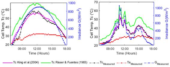
Fig. 5 Estimated Tc by the best and worst correlation model for clear sky (left) and cloudy sky (right) conditions 

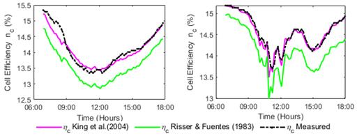
Fig. 6 Estimated efficiency ηc by the best and worst correlation model for clear sky (left) and cloudy sky (right) conditions 

In both figures are verified that the irradiance G significantly influences the temperature of cell Tc, increasing and decreasing Tc according to the trend of G for each day represented. In the case of figure 6, it can be seen how the efficiency is higher the morning and the afternoon hours, reaching lower values in the midday hours, this is mainly due to the temperature of operation variation Tc. As the zenith approaches, the irradiance increases and consequently the operating temperature of the photovoltaic modules, which causes a maximum attenuation of efficiency ηc. This behavior is similar both on clear sky days and on cloudy days.

For the date October 27, 2018, the King et al. (2004) model has an efficiency at range of 15.18% - 13.49%, while Risser & Fuentes (1983) model was at range of 14.95%. - 12.98%. For the date January 30, 2019, the King et al. (2004) model has an efficiency at range of 15.23% - 13.41%, while the Risser & Fuentes (1983) model was at range of 14.76% - 12.85%. For both models, an energy efficiency value of PV modules was obtained below that established by the manufacturer at the technical datasheet, for clear sky conditions and also for cloudy sky conditions.

The statistical coefficients described above to assessment the two models are presented in table 7.

Table 7 Statistical coefficients of the best and worst correlation model 

Models	Day October 27, 2018 (clear sky)			Day January 30, 2019 (cloudy sky)
	R^2	RMSE (°C)	MAE (°C)	R^2	RMSE (°C)	MAE (°C)
King et al. (2004)	0.947	2.672	2.447	0.943	1.862	1.219
Risser & Fuentes (1983)	0.937	2.919	10.648	0.932	2.039	8.684

For analized days, the King et al. (2004) model had a better correlation than Risser & Fuentes (1983). The difference at MAE coefficient of both models is notable, while the coefficients of R² and RMSE showed less difference.

Conclusions

The estimation of the operating temperature is very important for sizing and economic technical studies, because it improves the estimation of the energy efficiency of PV systems. The Tc measurements at the CIES in Santiago de Cuba are higher than the 25 °C defined in PV module technical datasheet, so it’s important to know the effect of Tc on the ηc of the PV cell. In this study, 10 models were assessed, from which it’s concluded:

• The variables that correlated with the cell temperature Tc were the irradiance G, the ambient temperature Ta and the wind speed v, the King et al. (2004) model presented the best accuracy criteria, whit coefficientes R²=0.912, RMSE=3.482 °C and MAE=2.698 °C.

• The King et al. (2004) model estimates the temperature Tc and it’s effect on the efficiency of the module, in such a way that the increase of 1 °C causes a decrease effect of -0.042 at the efficiency ηc of the PV cell. This linear relationship correctly estimates the energy behavior of the CIES modules for various weather conditions. For the months studied (September 2018 to March 2019), the efficiency dropped to 1.9% during the day, so in summer months it should decrease even more.

• Although the study only includes monocrystalline silicon technology, in a period of time that does not cover the 12 months of year, the results are valid to know the effect of Tc on the efficiency of the PV modules installed in Santiago de Cuba.

According to the 2021 Statistical Yearbook of Cuba, the temperatures between provinces do not have a considerable difference, that why this study could be taken as a reference for any other region of the country for PV system projects ^[44]. As a future perspective, it’s planned to extend the study to other areas of Cuba and other PV technologies such as amorphous silicon and polycrystalline silicon, in order to establish a more accurate model that improves the estimate of Tc.

References

1.  International Energy Agency. “Renewable Energy Market Update”. Outlook for 2021 and 2022. International Energy Agency, 2022, vol., p. 29. Available at: https://iea.blob.core.windows.net/assets/18a6041d-bf13-4667-a4c2-8fc008974008/RenewableEnergyMarketUpdate-Outlookfor2021and2022.pdf1.

2.  Feldman, David, et al. “Winter 2021/2022 Solar Industry Update”. National Renewable Energy Laboratory’s (NREL). 2022, vol., p. 51. Available at: https://www.nrel.gov/docs/fy22osti/81900.pdf2.

3.  IRENA. “Renewable Energy Statistics 2021”. The International Renewable Energy Agency, Abu Dhabi. 2021. Available at: www.irena.org/2021/publications/Aug/Renewable-energy-statistics-20213.

4.  Raynel, Díaz Santos, et al. “Análisis de la influencia del ángulo de inclinación en la generación de una central fotovoltaica”. Revista de Ingeniería Energética, 2018, vol. 39, n. 3, p. 146-156. Available at: http://scielo.sld.cu/pdf/rie/v39n3/rie02318.pdf4.

5.  Gutiérrez Urdaneta, Luis; Padrón Suárez, Lenyer; Valladares Aguilera, J. “Marginal contribution of factors to energy gains of bifacial modules”. Ingeniería Energética, 2021, vol. , n.1, e2912, 2021, vol. 42 (1, enero/abril), p. 1-12. Available at: https://rie.cujae.edu.cu/index.php/RIE/article/view/608/pdf5.

6.  Gutiérrez Urdaneta, Luis; Padrón Suárez, Lenyer; Valladares Aguilera, J. “Una revisión de la distancia entre filas de los parques fotovoltaicos con limitaciones de terreno”. Ingeniería Energética , 2021, vol. 42, n. 2, mayo/agosto. p. 1-11. Available at: https://rie.cujae.edu.cu/index.php/RIE/article/view/6186.

7.  Gutiérrez Urdaneta, Luis , et al. “Sistemas de ajuste manual de inclinación de paneles fotovoltaicos y de seguimiento automático horizontal de un eje”. Ingeniería Energética , 2020, vol. 41, n. 2, p. 1-11. Available at: http://scielo.sld.cu/scielo.php?script=sci_arttext&pid=S1815-590120200002000027.

8.  Korkeakoski, Mika. “Towards 100% Renewables by 2030: Transition Alternatives for a Sustainable Electricity Sector in Isla de la Juventud, Cuba”. Energies, 2021, vol. 14 (2862), p. 1-22. Available at: https://doi.org/10.3390/en141028628.

9.  Alberto Alvarez, Ernesto, et al. “Long-Range Integrated Development Analysis: The Cuban Isla de la Juventud Study Case”. Energies , 2021, vol. 14, n. 10, p. 2865. Available at: https://doi.org/10.3390/en141028659.

10.  Schwingshackla, C., et al. “Wind effect on PV module temperature: Analysis of different techniques for an accurate estimation”. Energy Procedia, 2013, vol. 40, p. 77 - 86. Available at: https://dx.doi.org/10.1016/j.egypro.2013.08.01010.

11.  Meral, M. E. y Dincer, F. “A review of the factors affecting operation and efficiency of photovoltaic based electricity generation systems”. Renewable and Sustainable Energy Reviews, 2011, vol. 15, n. 5, p. 2176-2184. Available at: https://doi.org/10.1016/j.rser.2011.01.01011.

12.  Bayrak, F, et al. “A review on exergy analysis of solar electricity production”. Renew. Sustain. Energy Rev, 2017, vol. 74, p. Available at: https://www.doi.org/10.1016/j.rser.2017.03.01212.

13.  Green, M. A, et al. “High-Efficiency silicon solar cells”. IEEE Trans. Electron Devices, 1984, vol. 1984 n. 31, p. 679-683. Available at: https://doi.org/10.1109/T-ED.1984.2158913.

14.  Skoplaki, E, et al. “A simple correlation for the operating temperature of photovoltaic modules of arbitrary mounting”. Solar Energy Materials and Solar Cells, 2008, vol. 92, n. 11, p. 1393-1402. Available at: https://doi.org/10.1016/J.SOLMAT.2008.05.01614.

15.  Mukisa, N; Zamora, R; Lie, T. T. “Analysis of Solar Cell Temperature Models used in Solar Photovoltaic Simulating Softwares”. Proceedings of the 2019 IEEE PES GTD Asia, 2019. Available at: http://dx.doi.org/10.1109/GTDAsia.2019.871591615.

16.  Zouine, M, et al. “Confrontation with the Experience of 48 Combinations of Models of the Thermal and Electrical Behavior of Crystalline Solar Modules”. International Journal Of Renewable Energy Research, 2021, vol. 11, n. 1, p. 426-439. Available at: https://www.ijrer.org/ijrer/index.php/ijrer/article/view/11796/pdf16.

17.  Liao, Wei, et al. “Evaluation of Temperature Dependent Models for PV Yield Prediction”. [en línea]. En: 4th Building Simulations and Optimizations Conference. International Building Simulation Association. Cambridge, United Kingdom. 2018, p. 8. Available at: http://www.ibpsa.org/bso-2018-proceedings/17.

18.  Nguyen, Dang Phuc Nguyen; Neyts, Kristiaan; Lauwaert, Johan. “Proposed Models to Improve Predicting the Operating Temperature of Different Photovoltaic Module Technologies under Various Climatic Conditions”. Appl. Sci., 2021, vol. 11, n. 15, p. 1-14. Available at: https://doi.org/10.3390/app1115706418.

19.  Umoette, Anyanime Tim; Ubom, Emmanuel A.; Akpan, Ibiangake Etie. “Comparative Analysis of Three NOCT-Based Cell Temperature Models”. International Journal of Systems Science and Applied Mathematics, 2016, vol. 1, n. 4, p. 69-75. Available at: https://doi.org/10.11648/j.ijssam.20160104.1619.

20.  Munoz, M. A, et al. ``Early degradation of silicon PV modules and guaranty conditions”. Solar energy 2011, vol. 85, n. 9, p. 2264-2274. Available at: https://doi.org/10.1016/j.solener.2011.06.01120.

21.  Ya'acob, M. Effendy; et al. “Modelling of photovoltaic array temperature in a tropical site using generalized extreme value distribution”. Journal of Renewable and Sustainable Energy, 2014, vol. 6, p. 9. Available at: http://dx.doi.org/10.1063/1.488517521.

22.  Duffie, John A y Beckman, William A. “Solar Engineering of Thermal Processes”. Wiley 4. Wiley 4 th., 2013. Available at: https://www.wiley.com/en-us/Solar+Engineering+of+Thermal+Processes,+4th+Edition-p-978047087366322.

23.  Sredenšek, Klemen, et al. “Experimental Validation of a Thermo-Electric Model of the Photovoltaic Module under Outdoor Conditions´´. Applied Sciences, 2021, vol. 11, p. 1. Available at: https://doi.org/10.3390/app1111528723.

24.  Lawrence Kamuyu, Waithiru Charles; et al. “Prediction Model of Photovoltaic Module Temperature for Power Performance of Floating PVs”. Energies , 2018, vol. 11, p. 8. Available at: https://doi.org/10.20944/preprints201712.0094.v124.

25.  King, David L, et al. Report: “Photovoltaic array performance model” No: SAND2004-3535, 2004, vol. 8, p. 1-19. Available at: https://doi.org/10.2172/91913125.

26.  Faiman, David. “Assessing the Outdoor Operating Temperature of Photovoltaic Modules”. Progress in Photovoltaics: Research And Applications, 2008, vol. 16, p. 307-315. Available at: https://doi.org/10.1002/pip.81326.

27.  Koehl, M, et al. “Modeling of the nominal operating cell temperature based on outdoor weathering”. Solar Energy Materials and Solar Cells 2011, vol. 95, n. 7, p. 1638-1646. Available at: https://doi.org/10.1016/j.solmat.2011.01.02027.

28.  Akhsassi, M, et al. “Experimental investigation and modeling of the thermal behavior of a solar PV module”. Sol. Energy Mater. Sol. Cells, 2018, vol. 180, p. 271-279. Available at: https://doi.org/10.1016/j.solmat.2017.06.05228.

29.  Coşkun, Can, et al. “Estimation of pv module surface temperature using artificial neural networks”. Mugla Journal of Science and Technology, 2016, vol. 2, n. 2, p. 15-18. Available at: https://doi.org/10.22531/MUGLAJSCI.28361129.

30.  Chandra, Subhash; Yadav, Arvind; Chauhan, D.S. “Experimental investigation to obtain the pv module true performance and emphasis on application of soft computing”. International Journal of Advanced Science and Technology 2019, vol. 28, n. 14, p. 285-297. Available at: http://sersc.org/journals/index.php/IJAST/article/view/149330.

31.  Chandra, Subhash; Agrawal, Sanjay; Chauhan, D.S. “Soft computing based approach to evaluate the performance of solar PV module considering wind effect in laboratory condition”. Energy Reports, 2018, vol. 4, p. 252-259. Available at: http://dx.doi.org/10.1016/j.egyr.2017.11.00131.

32.  Bassam, A., et al. “Temperature Estimation for Photovoltaic Array Using an Adaptive Neuro Fuzzy Inference System”. Sustainability, 2017, vol. 9, p. 1-16. Available at: https://doi.org/10.3390/su908139932.

33.  Risser, V. V y Fuentes, M. K. “Linear regression analysis of flat-plate photovoltaic system performance data”. In 5th Photovoltaic Solar Energy Conference. 1984. Available at: https://ui.adsabs.harvard.edu/abs/1984pvse.conf.623R/abstract33.

34.  Muzathik, A. M. “Photovoltaic modules operating temperature estimation using a simple correlation”. International Journal of Energy Engineering, 2014, vol. 4, n. 4, p. 151. Available at: https://www.researchgate.net/publication/26791100034.

35.  Proenza Yero, Roger; Emilio Camejo, José; Ramos Heredia, Rubén. “Modeling and simulation of a grid-connected photovoltaic system”. IJRDO - Journal of Electrical And Electronics Engineering, 2019, vol. 5, n. 2, p. 1-8. Available at: https://www.ijrdo.org/index.php/eee/article/view/2701/224835.

36.  HELIENE. HELIOS ENERGY EUROPE S.L. ``Módulos Solar HEE215M´´. 2012, vol., p. 2. Available at: http://avdira-solar.eu/pdf/heliene/215m_en.pdf36.

37.  Yang, Renata Lautert, et al. “Photovoltaic Cell Temperature Estimation for a Grid-Connect Photovoltaic Systems in Curitiba”. Brazilian Archives Biology and Tecnology, 2019, vol. 62 (e19190016), p. 1-9. Available at: https://dx.doi.org/10.1590/1678-4324-smart-201919001637.

38.  Jatoi, Abdul Rehman; Samo, Saleem Raza; Jakhrani, Abdul Qayoom. “An Improved Empirical Model for Estimati on of Temperature Effect on Performance of Photovolta ic Modules”. International Journal of Photoenergy, 2019, vol. 2019, p. 1-16. Available at: https://doi.org/10.1155/2019/168135338.

39.  Ross, R.G y Smokler, M. I. “Flat-plate solar array project. Volume 6: Engineering sciences and reliability”. Report DOE/JPL-1012-125; California, United States of America. 1986. Available at: https://ntrs.nasa.gov/citations/1987001121839.

40.  Eckstein, Jürgen Helmut. “Detailed Modelling of Photovoltaic System Components”. Master Thesis. University of Wisconsin-Madison, 1990. Available at: https://minds.wisconsin.edu/bitstream/handle/1793/45596/Eckstein1990.pdf40.

41.  Mattei, M, et al. “Calculation of the polycrystalline PV module temperature using a simple method of energy balance´´. Renewable Energy, 2006. p. 553-567. Available at: https://doi.org/10.1016/j.renene.2005.03.01041.

42.  Skoplaki, E y Palyvos, J. A. “On the temperature dependence of photovoltaic module electrical performance: A review of efficiency/power correlations”. Solar energy , 2009, vol. 83, n. 5, p. 614-624. Available at: https://doi.org/10.1016/j.solener.2008.10.00842.

43.  Idzkowski, Adam; Karasowska, Karolina; Walendziuk, Wojciech. “Temperature Analysis of the Stand-Alone and Building Integrated Photovoltaic Systems Based on Simulation and Measurement Data”. Energies , 2020, vol. 13, p. 1-21. Available at: https://doi.org/10.3390/en1316427443.

44.  ONEI. Oficina Nacional de Estadísticas e Información. Anuario Estadístico de Cuba 2020. Capítulo 2: Medio Ambiente. Edición 2021. 2021. p. 62. Available at: http://www.onei.gob.cu/sites/default/files/02_medio_ambiente_0.pdf44.

Received: October 04, 2022; Accepted: November 05, 2022

^* Autor de correspondencia: [e-mail]

The authors declare that there are no conflicts of interest

M.Sc. Liomnis Osorio Laurencio: Responsible of the idea and design of the state of art. Data processing and analysis and interpretation of research. Review of references. Programming of the computational tool of the methods used. Writing and final review of research.

Dr. C. Yoalbys Retirado-Mediaceja: Methodological design and organization of research. Writing of the research methods and instrumentation used. Programming at the computational tool of the used methods. Revision of final report.

Ing. José Emilio Camejo Cuán: collection and analysis. Writing of the research methods and instrumentation used. Analysis of results obtained in research. Final report review and approval.

M.Sc. Roger Proenza Yero: Measurement collection and analysis. Writing of the research methods and instrumentation used. Analysis of results obtained in research. Final report review and approval.

M.Sc. Adrián Romeu Ramos: Measurement collection and analysis. Writing of the research methods and instrumentation used. Analysis of results obtained in research. Final report review and approval.

Ing. Eliannet Varga Estupiñan: Measurement collection and analysis. Writing of the research methods and instrumentation used. Analysis of results obtained in research. Final report review and approval