Artículo original

Classifier ensemble algorithm for learning from non-stationary data stream

Ensamble de clasificadores para el aprendizaje a partir de flujos de datos no estacionarios.

Alberto Verdecia Cabrera^{1  *}  , Isvani Frías Blanco²  , Agustín Ortiz Diaz³  , Yanet Rodríguez Zarabia⁴  , Héctor Raúl González Diez⁵ 

¹Departamento de Informática. Universidad de Granma

²LexisNexis Risk Solutions. Sao Paulo, Brazil

³CCT-UDESC Santa Catarina State University, Joinville, Santa Catarina, Brazil

⁴Centro de investigaciones de la informática. Universidad Central Marta Abreu de las Villas

⁵Universidad de las Ciencias Informáticas, La Habana, Cuba

ABSTRACT

Nowadays, many sources generate unbounded data streams at high incoming rates. It is impossible to store these large volumes of data and it is necessary to process them in real time. Because these data are acquired over time and the dynamism of many real world situations, the target function to be learned can change over time, a problem commonly called concept drift. This paper presents a new ensemble algorithm called Classifier Ensemble Algorithm (CEA), able for learning from data streams with concept drift. CEA manipulates these changes using a change detector in each base classifier. When the detector estimates a change, the classifier in which the change was estimated is replaced by a new one. CEA combines the simplicity of the bagging algorithm to train base classifiers and Exponentially Weighted Moving Average (EWMA) control charts to estimate the weights of each base classifier. The proposed algorithm is compared empirically with several bagging family ensemble algorithms able to learn from concept-drifting data. The experiments show promising results from the proposed algorithm (regarding accuracy), handling different types of concept drifts.

Key words: classifier ensemble; concept drift; data stream

RESUMEN

En la actualidad, muchas fuentes generan flujos de datos ilimitados a altas tasas de entrada. Es imposible almacenar estos grandes volúmenes de datos por lo que es necesario procesarlos en tiempo real. Debido a que estos datos se adquieren a lo largo del tiempo y la dinámica de muchas situaciones reales, la función objetivo que se debe aprender puede cambiar con el tiempo, un problema que comúnmente conocido como cambio de concepto. En este artículo se presenta un nuevo algoritmo de ensamble denominado Algoritmo de Ensamble de Clasificadores (CEA), capaz de aprender de flujos de datos con cambios de concepto. CEA manipula estos cambios utilizando un detector de cambios en cada clasificador base. Cuando el detector estima un cambio, el clasificador en el que se estimó el cambio se reemplaza por uno nuevo. CEA combina la simplicidad del algoritmo de bagging para entrenar clasificadores base y el esadístico EWMA para estimar los pesos de cada clasificador base. El algoritmo propuesto se compara empíricamente con varios algoritmos de ensamble basados en bagging capaces de aprender de flujos de datos con cambios de concepto. Los experimentos muestran que el algoritmo propuesto muestra resultados prometedores (con respecto a la precisión), manipulando diferentes tipos de cambios de concepto.

Palabras-clave: cambio de concepto; ensamble de clasificadores; flujos de datos

INTRODUCTION

The volume of data generated by sensors, Internet, location devices, cell-phones, and many others is constantly increasing. The size of this data is potentially infinite, due to its constant generation and thus, it is necessary to process them with limited computational resources. The use of machine learning techniques is a viable option for this processing. Machine learning can be classified into two types, depending on how the training examples are presented (^{Nishida, 2008}): batch learning and online learning. A batch learning system is first given a large number of examples and then learns them all at once. In contrast, an online learning system is given examples sequentially and learns them one by one. In classification tasks, a data stream is commonly defined as a very large (potentially infinite) sequence of pairs that are acquired over time. These pairs, called instances or examples, are composed of a set of attributes and a class label. Because of the temporal dimension of the data, and the dynamism of many real-world situations, the target function to be learned can change over time, a problem commonly known as concept drift. Consequently, the learning algorithms must be updated with respect to the most recent concepts (^{Gama et al., 2014}).

Classifier ensembles have been successfully used for mining data streams (^{Zang et al., 2014}; ^{Ortíz Díaz et al., 2014}; ^{Ghomeshi et al., 2019}). Ensemble methods combine the predictions from base classifiers aiming at improving the predictive accuracy obtained by a single classifier. Classifier ensembles require three main components in their design (^{Kuncheva, 2004}): (1) a method for training the base classifiers, (2) a voting procedure, and (3) the base learning algorithms. However, in order to deal with concept drift, previous ensemble methods have principally been focused on modifying the structure of the ensemble. They have used performance measures to monitor the ensemble consistency regarding new data. Significant variations in the performance values are interpreted as a concept drift, and the ensemble algorithms eliminate, reactivate or add new base classifiers dynamically in response to these variations (^{Bifet et al., 2009}, 2010b; ^{Frías-Blanco et al., 2016}; ^{Verdecia-Cabrera et al., 2018}).

For example, ^{Oza and Russell (2001}) proposed online bagging and boosting methods for training base classifiers, assuming that concepts are stationary. Online bagging can straightforwardly be applied to learning from instances. Examples of algorithms based on online bagging include OzaBagADWIN and LeveragingBag (^{Bifet et al., 2009}, 2010b), which use the ADWIN algorithm (^{Bifet, 2010}) for change detection and error estimates. When a change is detected, the worst classifier in the ensemble is removed and a new classifier is added to the ensemble. Even though these algorithms are able to learn from non-stationary data, they do not handle concept drift explicitly in the base classifiers.

This motivated us to present a new ensemble method, named Classifier Ensemble Algorithm (CEA), for data stream classification with concept drift. CEA combines the simplicity of the online bagging algorithm (^{Oza and Russell, 2001}) and the EWMA (Exponentially Weighted Moving Average) method (^{Hunter and others, 1986}) to weight the base classifiers. To manipulate changes in concept in the base classifiers CEA uses Hoeffding- based Drift Detection Method (HDDM) (^{Frias-Blanco et al., 2015}) for drift detection and error estimates, which monitors error rates in order to trigger three different drift signals during the learning process. HDDM triggers the in-control signal when the current concept remains stable, warning when a concept drift is likely to be approaching, and out-of-control when a concept drift is detected. So, when the detector estimates a change, the classifier in which the change was detected is replaced by a new one. To train the base classifiers, we use previous online bagging.

MATERIALS Y METHODS

Concept drift

In online learning, a classification task is generally defined for a sequence (possibly infinite) of instances S = e1, e2, .., ei,... arriving over time. Every training instance is formed by a vector and a discrete value yi. Each vector has the same dimensions. Each dimension is named attribute and each component is an attribute value (numeric or symbolic). The discrete value yiis named label and taken from a finite set Y of possible class values.

It is commonly assumed that the data stream S is generated by a probability density function The classification learning task is to obtain a model from S that approximates P as so that maximizes the predictive accuracy (^{Verdecia-Cabrera et al., 2018}). Concept refers to the probability distribution function of the problem at a given time stamp. Therefore, a change in P after a time stamp entails a concept change or concept drift. ^{Gama et al. (2014}) distinguish two main types of concept drift:

• Real concept drift refers to changes in the distribution of posterior probability of the classes P (Y | X). These changes can occur without a change in the probability distribution of the instance space P (X).

• Virtual concept drift happens when the probability distribution of the instance space changes (P (X))

^{Stanley (2003}) recognizes two types of changes related to the frequency with which the instances that describe the new concept are received: abrupt and gradual. An abrupt change occurs when the transition between consecutive concepts is instantaneous. A gradual change occurs when the transition period between consecutive concepts contains a certain number of training instances.

Classifier ensemble algorithm

In this section, we present a new classifier ensemble in combination with online bagging and EWMA, able to learn from non-stationary data streams.

Online version of the bagging algorithm

Bagging (^{Breiman, 1996}) is an ensemble methods used to train and improve the accuracy of classifier methods. Non-streaming (^{Breiman, 1996}) bagging builds a set of M base models, training each model with a bootstrap sample of size N created by drawing random samples with replacement from the original training set. Each base model’s training set contains each of the original training examples K times where P (K = k) follows a binomial distribution. This binomial distribution for large values of N tends to a Poisson(1) distribution, where P (1) = exp (−λ) /k!. Using this fact, ^{Oza and Russell (2001}) proposed Online Bagging, an online method that instead of sampling with replacement, gives each example a weight according to Poisson (1). So, the proposed method in this paper uses online bagging algorithm to train base classifiers.

EWMA

EWMA (Exponentially Weighted Moving Average) is a method of Statistical processes control. The essential feature of this method is that it gives more weight to the most recent observations. The statistic that is represented in the chart is:

where

xi	is a random variable
β	is a constant to determine the weight of the observations, (0 < β < 1)
Wi	is the current value of EWMA
Wi−1	is the previous value.

In this work, the equation 1 is used to determine the weight of the base classifiers. In this case, Wiis the weight of each classifier and xi the current accuracy. As each classifier uses a change detector, it can be estimated at any time the error Em of each base classifier and the accuracy is 1 − Em.β can be used as a factor to adjust the weights of the base classifiers.

The new algorithm

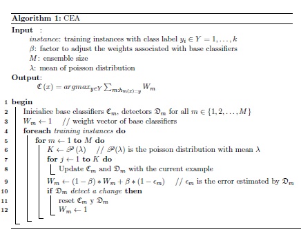
The proposed algorithm called CEA uses the online version of the bagging algorithm to train the base classifiers and the EWMA method to determine the weights of the classifiers. CEA manipulate concept changes in a simple and efficient way (see algorithm 1). Each base classifier Cm (1 < m < M ) uses a change detector to estimate the error rate Em of each classifier. When estimate a change, the Cm classifier is replaced by a new one. To estimate the weight of each classifier, we used the equation 1. The algorithm receives as parameters the number of base classifiers and the factor β to adjust the weights associated in the base classifiers. The higher value of β, greater importance is given to the most recent data.

The error rate of the base classifiers is monitored constantly as each training example arrives. Therefore, this monitoring must also be done with resources controlled computational. In recent years have been proposed several methods in the statistical community to detect changes online (^{Montgomery, 2007}). However, they assume that the input data are regulated by a known probability distribution. CEA uses HDDM (Hoeffding Drift Detection Method) (^{Frias-Blanco et al., 2015}) as change detector and error estimates. HDDM processes each incoming value with a constant time and space complexity and provides mathematical guarantees for the false positive and false negative rates.

RESULTS Y DISCUSSION

Empirical Study

This section experimentally compared CEA with various state-of-the-art ensemble algorithms for mining concept-drifting data streams. The experiments measured the generalization power of the contending algorithms by means of predictive accuracy (^{Bifet et al., 2010}a). Performance measures related with the computational cost were not considered, as the contending algorithms are able to learn with constant time and space computational complexity per instance processed.

All the experiments were implemented and performed using the Massive Online Analysis (MOA) software (^{Bifet et al., 2010}a). MOA includes a collection of algorithms for processing data streams, various methods to generate artificial data streams with the possibility of including concept drifts, and several tools to evaluate concept drift detection algorithms.

The algorithms under consideration were evaluated by a test-then-train approach, which is derived from the predictive sequential error (^{Dawid, 1984}). Test-then-train computes the predictive performance of a learning model as each training instance arrives (test step). In the next step, the instance is presented to the learning algorithm for learning (train step). This methodology is based on the cumulative sum of the values of a given function. We calculated metrics by means of a sliding window considering only the last instances (^{Gama et al., 2009}). Therefore, at each new instance, the classifier was first tested and then trained. During the learning process, predictive accuracy was calculated with respect to a sliding window of size 100 (^{Bifet et al., 2010}a). Predictive accuracy was calculated every 100 instances processed by means of the fraction between the number of correctly classified instances and the window’s size.

Datasets

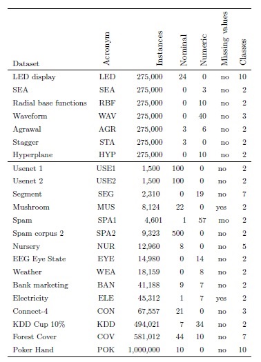
The experiments considered both artificial (LED, SEA, RBF, WAV, AGR, STA, HYP) and real-world datasets (see Table 1). The artificial datasets have the benefit of modeling different scenarios where the algorithms can demonstrate their performance. We can distinguish two types of datasets, those that are oriented to test abrupt changes, and those that introduce gradual changes. Furthermore, other characteristics can be added, like artificial noise, irrelevant attributes, etc. Regarding abrupt datasets, the common idea that supports their operation is the generation of distinct concepts that are active in different periods. The change between concepts is immediate (abrupt change), although the extent of the change could simulate a gradual change in some way. Thus, if two consecutive concepts are very similar, it could be considered that the speed of the change is low. The artificial datasets were generated by the MOA software (^{Bifet et al., 2010}a).

Table 1 Main characteristics of the datasets used in the experiments. 

In the artificial datasets, the target concept changed 10 times. Changes occurred every 25, 000 instances. In gradual changes, the transition period between consecutive concepts was set to 5, 000 training instances. During the transition period, the probability that a new training instance belongs to the new concept was increased gradually and continuously.

Algorithm Setup

The proposed CEA algorithm was compared with the algorithms based on online bagging. The algorithms used in the experimental study are available in MOA. Specifically, included ^{OzaBag (online version of the bagging algorithm) (Oza and Russell, 2001}), OzaBagAdwin (^{Bifet et al., 2009}) and LeveragingBag (^{Bifet et al., 2010b}). The contending algorithms were set with the default configuration adopted by MOA (^{Bifet et al., 2010a}). In the case of CEA we use λ = 6, and β = 0.875. The number of classifiers of the contending algorithms in MOA is 10. Therefore, in CEA the number of classifiers was set to 10.

All the contending algorithms used Naive Bayes as a base classifier. Naive Bayes was chosen because it is one of the most successful algorithms for learning from data streams (^{Clark and Niblett, 1989}; ^{Cestnik and others, 1990}; ^{Domingos and Pazzani, 1997}; ^{Pereira-Toledo et al., 2017}): it has a low computational cost, is simple, has a clear semantics, and works well with continuous attributes and missing attribute values. In the drift detection method of CEA, the size of the statistical test for the warning level was set to = 0.005, and the drift level was set to = 0.001; this configuration allowed a balance between the false positive rate, false negative rate, and delay of change detections.

Results

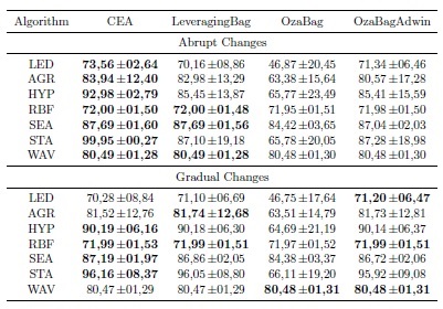
The Table 2 summarize the predictive performance of the algorithms over abrupt and gradual changes in terms of the average and standard deviation. The highest levels of predictive accuracy are in bold. The Table 2 reflects that the proposed algorithm often outperformed the algorithms LeveragingBag, OzaBag, and OzaBagAdwin. In RBF and SEA, consecutive concepts were configured to be very similar. Additionally, the Figure 1 reflects that CEA is often able to adapt to concept drifts more quickly than the contending algorithms. We can also see that CEA is able to stabilize the learning when concepts are stable.

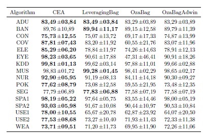
The concept drift problem can be more adverse in real-world situations. The real world datasets included in this section have been used in several studies on concept drift (Table 1). For these datasets, there is no strong claim about the presence or type of change. Similar to the results obtained from the synthetic datasets, CEA often reached higher levels of predictive accuracy and when outperformed, its accuracy was very similar to that of the winner. Figure 2 shows the ranking position of the algorithms with respect to Table 2 and Table 3. To verify significant differences, we used the Friedman test and the Holm procedure for the post hoc analysis. Groups of classifiers that are not significantly different (at p = 0.05) are connected. This figure shows that, in general, CEA ranked significantly better than the contending algorithms, excepting LeveragingBag.

Table 2 Predictive performance of the algorithms in abrupt and gradual changes. 

Table 3 Predictive performance of the algorithms in real datasets. 

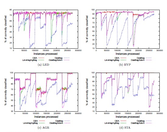
Fig. 1 Accuracy of the contending algorithms with abrupt changes. Changes occur every 25,000 instances. 

Fig. 2 Comparison of all classifiers against each other with the Friedman test and the Holm method for the post hoc analysis. Groups of classifiers that are not significantly different (at p = 0:05) are connected. The ranks were computed in accordance with Table 2 and Table 3. 

CONCLUSIONS

In this paper we have presented Classifier Ensemble Algorithm (CEA), a new algorithm able to learn from non- stationary data streams. The new algorithm combines the simplicity of online bagging to train base classifiers and the EWMA method to estimate the weights of the base classifiers. The new algorithm process stream data in constant time and space computational complexity, and can learn with a single scan over the training data. CEA uses an online change detector for drift detection and error estimates. When the detector estimates a change, the classifier in which the change was detected is replaced by a new one. CEA was compared empirically with ensemble algorithms based on online bagging. All the algorithms were tested against the common types of changes (abrupt and gradual), different noise levels and irrelevant attributes. The experiments showed that the new algorithm is an efficient alternative for learning from data streams.

We plan to continue with this research by using other learning algorithms as base classifiers in CEA, such as Hoeffding trees and Perceptron.

REFERENCES

Bifet, A. (2010). Adaptive Stream Mining: Pattern Learning and Mining from Evolving Data Streams. In Proceedings of the 2010 Conference on Adaptive Stream Mining: Pattern Learning and Mining from Evolving Data Streams, pages 1-212, Amsterdam, The Netherlands, The Netherlands. IOS Press.

Bifet, A., Holmes, G., Kirkby, R., and Pfahringer, B. (2010a). Moa: Massive online analysis. The Journal of Machine Learning Research, 11:1601-1604.

Bifet, A., Holmes, G., and Pfahringer, B. (2010b). Leveraging bagging for evolving data streams. In Machine learning and knowledge discovery in databases, pages 135-150. Springer.

Bifet, A., Holmes, G., Pfahringer, B., Kirkby, R., and Gavalda, R. (2009). New ensemble methods for evolving data streams. In Proceedings of the 15th ACM SIGKDD international conference on Knowledge discovery and data mining, 2009, pages 139-148. ACM.

Breiman, L. (1996). Bagging predictors. Machine learning, 24(2):123-140.

Cestnik, B. and others (1990). Estimating probabilities: a crucial task in machine learning. In ECAI, volume 90, pages 147-149.

Clark, P. and Niblett, T. (1989). The CN2 induction algorithm. Machine learning , 3(4):261-283.

Dawid, A. P. (1984). Present Position and Potential Developments: Some Personal Views: Statistical Theory: The Prequential Approach. Journal of the Royal Statistical Society. Series A (General), 147(2):278-292.

Domingos, P. and Pazzani, M. (1997). On the optimality of the simple Bayesian classifier under zero-one loss. Machine learning , 29(2-3):103-130.

Frias-Blanco, I., Campo-Avila, J. d., Ramos-Jimenez, G., Morales-Bueno, R., Ortiz-Diaz, A., and Caballero- Mota, Y. (2015). Online and Non-Parametric Drift Detection Methods Based on Hoeffding Bounds. IEEE Transactions on Knowledge and Data Engineering, 27(3):810-823.

Frías-Blanco, I., Verdecia-Cabrera, A., Ortiz-Díaz, A., and Carvalho, A. (2016). Fast adaptive stacking of ensembles. In Proceedings of the 31st Annual ACM Symposium on Applied Computing, pages 929-934. 2009, ACM.

Gama, J., Rodrigues, P. P., and Sebastiao, R. (2009). Evaluating algorithms that learn from data streams. In Proceedings of the 2009 ACM Symposium on Applied Computing (SAC), Honolulu, Hawaii, USA, March 9-12, 2009, pages 1496-1500. ACM.

Gama, J., Zliobaite, I., Bifet, A., Pechenizkiy, M., and Bouchachia, A. (2014). A Survey on Concept Drift Adaptation. ACM Comput. Surv., 46(4):44:1-44:37.

Ghomeshi, H., Gaber, M. M., and Kovalchuk, Y. (2019). Ensemble Dynamics in Non-stationary Data Stream Classification. In Sayed-Mouchaweh, M., editor, Learning from Data Streams in Evolving Environments: Methods and Applications, Studies in Big Data, pages 123-153. Springer International Publishing, Cham.

Hunter, J. S. and others (1986). The exponentially weighted moving average. J. Quality Technol., 18(4):203-210.

Kuncheva, L. I. (2004). Combining pattern classifiers: methods and algorithms. John Wiley & Sons. .

Nishida, K. (). Learning and detecting concept drift. PhD thesis, School of Information Science and Technology, 2008, Hokkaido University.

Ortíz Díaz, A., del Campo-Ávila, J., Ramos-Jiménez, G., Frías Blanco, I., Caballero Mota, Y., Mustelier Hechavarría, A., and Morales-Bueno, R. (2014). Fast Adapting Ensemble: A New Algorithm for Mining Data Streams with Concept Drift. The Scientific World Journal.

Oza, N. C. and Russell, S. (2001). Online Bagging and Boosting. In Jaakkola, T. and Richardson, T., editors, Eighth International Workshop on Artificial Intelligence and Statistics, pages 105-112, Key West, Florida. USA. Morgan Kaufmann.

Pereira-Toledo, A., López-Cabrera, J. D., and Quintero-Domínguez, L. A. (2017). Estudio experimental para la comparación del desempeño de Naıve Bayes con otros clasificadores bayesianos. Revista Cubana de Ciencias Informáticas, 11(4):67-84.

Stanley, K. O. (2003). Learning concept drift with a committee of decision trees. Informe técnico: UT-AI- TR-03-302, Department of Computer Sciences, University of Texas at Austin, USA.

Verdecia-Cabrera, A., Blanco, I. F., and Carvalho, A. C. P. L. F. (2018). An online adaptive classifier ensemble for mining non-stationary data streams. Intelligent Data Analysis, 22(4):787-806.

Zang, W., Zhang, P., Zhou, C., and Guo, L. (2014). Comparative study between incremental and ensemble learning on data streams: Case study. Journal of Big Data, 1(1):5.

Montgomery, D. C. (2007). Introduction to statistical quality control. John Wiley & Sons

Received: August 29, 2018; Accepted: November 27, 2018

^*Autor para la correspondencia: [e-mail]