ARTÍCULO ORIGINAL

 

 

Optimizing grade-control drillhole spacing with conditional simulation

 

 

Espaciamiento óptimo de sondajes de control de leyes usando simulación condicional

 

 

 

Adrian Martínez Vargas¹

 

¹PhD in Geological Sciences. Principal Consultant. Opengeostat Consulting, Vancouver, British Columbia, Canada [e-mail]

 

 

 

---

Abstract

This paper summarizes a method to determine the optimum spacing of grade-control drillholes drilled with reverse-circulation. The optimum drillhole spacing was defined as that one whose cost equals the cost of misclassifying ore and waste in selection mining units (SMU). The cost of misclassification of a given drillhole spacing is equal to the cost of processing waste misclassified as ore (Type I error) plus the value of the ore misclassified as waste (Type II error). Type I and Type II errors were deduced by comparing true and estimated grades at SMUs, in relation to a cuttoff grade value and assuming free ore selection. True grades at SMUs and grades at drillhole samples were generated with conditional simulations. A set of estimated grades at SMU, one per each drillhole spacing, were generated with ordinary kriging. This method was used to determine the optimum drillhole spacing in a gold deposit. The results showed that the cost of misclassification is sensitive to extreme block values and tend to be overrepresented. Capping SMU’s lost values and implementing diggability constraints was recommended to improve calculations of total misclassification costs.

Keywords: drillhole spacing; conditional simulations; grade control.

 

---

Resumen

El artículo muestra un método para determinar el espaciamiento óptimo de sondajes de control de leyes perforados con circulación inversa. Como criterio de espaciamiento óptimo se tomó aquel cuyo costo iguala el costo de clasificar erróneamente de unidades de selectividad minera (SMU, siglas en inglés) en mena y estéril. El costo del error de clasificación, para un determinado espaciamiento entre sondajes, es igual al costo de procesar estéril erróneamente clasificado como mena (error Tipo I) más el valor de la mena clasificada erróneamente como estéril (error Tipo II). Los errores de Tipo I y II se dedujeron comparando los valores reales y estimados de las leyes en las SMU, en relación con una ley de corte determinada y asumiendo selección libre de las SMU mineralizadas. Los valores reales de las leyes en las SMU y en intervalos de muestreo de los sondajes se generaron con simulaciones condicionales. Los valores estimados en las SMU, uno para cada espaciamiento entre sondaje, se obtuvieron estimando con krigeage ordinario. El método propuesto fue usado para determinar el espaciamiento óptimo entre sondajes de un yacimiento de oro. Los resultados mostraron que el costo de clasificación errónea puede ser afectado por valores extremos en las SMU y tienden a ser sobrevalorados. Se propone usar topes en el valor del error de clasificación en las SMU y descartar las SMU no minables con el objetivo de reducir la sobreevaluación del valor total del error de clasificación.

Palabras clave: espaciamiento de la perforación; simulaciones condicionales; control de leyes.

---

 

 

 

1. INTRODUCTION

Classification of minable material into ore and waste, especially in open pit mining operations, is based on estimated grade in selection mining units (SMU). Estimated grades are obtained with interpolation from grade control drillholes, blast holes and channel data. The set of SMUs with interpolated grade is known as grade control model or short term model.

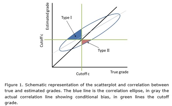
SMUs with interpolated grade over the cutoff are classified as ore, otherwise are classified as waste. A misclassification of ore and waste will occur if estimated and true grades are different and the cutoff grade is in between them, as shown in Figure 1. The SMU will be misclassified as ore and send to the mill (Type I error) if the true grade is below the cutoff and the estimate grade is over the cutoff (Figure 1). The SMU will be misclassified as waste and dump into waste piles (Type II error) if the true grade is over the cutoff but the estimate grade is below the cutoff (Figure 1).

The amount of misclassification is proportional to the conditional bias and the covariance between true and estimated grades. The percentages of SMU with Type I and II classification errors are not necessarily equal due conditional bias in interpolations, as shown in Figure 1. The best way to minimize misclassification is by reducing the space between grade control drillholes and carefully selecting interpolation parameters.

The optimum drillhole spacing is a problem investigated by many authors. Two approaches are used nowadays: (a) the drillhole spacing analysis (DHSA) and (b) drillhole spacing optimization with conditional simulations. The DHSA, as presented by Bertoli and other researchers (2013) and Verly, Postolski and Parker (2014), is based on the average kriging variance on SMUs in a mine production period. The DHSA does not provide a direct quantification of the cost of errors, the selection of the optimum spacing is based on an arbitrary percentage of interpolation error. The method can only be used on large areas. Bertoli et al. (2013) showed that results obtained with DHSA are similar to those obtained with conditional simulations.

Conditional simulations allow for a more direct estimation of the economic impact of extra drilling. Goria, Galli and Armstrong (2001) showed and example of the impact of extra drilling on global resources and reserve conversion. Boucher, Dimitrakopoulos and Vargas (2005) proposed a method where different drillhole spacing schemes are assessed with multivariate conditional simulations and economic indicators.

Most research work on drillhole spacing are focused on exploration drillholes, commonly used to build long term resource models. The most common criteria for selection of optimum spacing is the interpolation error required to classify resources into inferred, indicated and measure, as shown by Verly, Postolski and Parker (2014). There is not a consensus on the acceptable amount of interpolation error for a given mineral resource category. More tangible spacing criterion, like the cost of misclassification, are inappropriate to test spacing on exploration data because the selection will be base on future data, in other words, base on grade control drillholes.

The most commons grade control data in open pit mining operations come from blast holes and grade control reverse circulation (RC) drillholes. RC drillholes provide better sample quality but are more expensive and operationally more complex than blast holes. Incline RC drillholes provide better delineation of ore and waste in deposits with inclined and vertical structures.

This paper summarizes a method to determine the optimum spacing between grade control RC drillholes based on comparisons between misclassification costs and drilling costs.

  2. METHODS AND ASSUMPTIONS

Let’s assume that grade control samples will be collected from RC drillholes and samples and assays are representative of the style of the mineralization. In this case the optimum drillhole spacing is that one where the cost of drilling equals the cost of misclassifying a selective mining unit V. This can be expressed as shown in equation (1):

cost of drilling(S,m,l)-cost of misclassification(c,V,RF)=0                (1)

The cost of drilling is a function of the shape of the mineralization (S), the drillhole spacing (l) and the cost of each meter drilled (m). The shape S can be defined as an interpretation of the mineralization, usually represented by 3D wireframes. In practice the cost of drilling is calculated as the sum of lengths of sample intervals within S multiplied per the cost of drilling one unit of length.

The cost of misclassification is a function of the grade cutoff (c), the shape and size of the SMU (V) and the spatial random function describing grades in the interpolation domain (S). The cost of misclassification is calculated as shown in equation (2):

cost of misclassification = cost of Type I error + cost of Type II error           (2)

Where: cost of Type I error is the cost sending waste to the mill and cost of Type II error is the cost of sending ore to waste piles and are calculated as show in equations (3) and (4):

cost of Type I error = 1_{type I error}(block value – mining cost – processing cost)   (3)

cost of Type II error = 1_{type II error}(-block value-mining cost – processing cost) (4)

Where:

Note that the estimation errors only impact the values of the indicator functions of type I and type II classification errors. If grades are interpolated with ordinary kriging the interpolation errors depend on the random function model described by the variogram, drillhole spacing and SMU size, as explained by Chilès and Delfiner (2009). The interpolation errors may also depend on kriging plan and sample centroid locations.

To optimize drillhole spacing we need to obtain SMU’s true and estimated grades, the other cost variables in equations (2), (3) and (4) are assumed known and deterministic. True and estimated grades can be obtained using a simulation approach, as explained by Journel and Kyriakidis (2004).

The algorithm proposed to optimize drillhole spacing is as follow:

1. Obtain true and estimated grades on SMUs:

a. Simulate in a fine grid realistic realizations of the deposit using simulations conditioned with exploration drillhole data.

b. Reblock the fine grid to obtain true grades with SMU support.

c. Define RC drillhole paths at different spacing and resample from simulations in fine grid to generate RC sample intervals with simulated grades.

d. Estimate using grades on RC drillholes at different spacing to obtain SMU’s estimated grades.

2. Evaluate equations (2), (3) and (4):

a. Calculate type I and II errors and the cost of misclassification at different drillhole spacing.

b. Calculate the cost of RC drilling at different spacing.

c. Plot the total cost of drilling and cost of misclassification and define the optimum spacing.

This algorithm assumes free selection of ore and waste, which may be prohibitive for very small SMUs and isolated ore SMUs.

It is important to consider different simulation scenarios to assess variations in misclassification costs. For example, realizations generated with sequential Gaussian simulation (SGS) will show less connectivity between extreme grades and more spatial disorder than sequential indicator simulations (SIS) due to the maximum entropy property of SGS, as shown by Larrondo (2003). For this reason, SGS simulations will show higher cost of misclassification than SIS. Another way to assess variation is by using alternative geological interpretations as simulation domains (S).

3. DETERMINING THE OPTIMUM DRILLHOLE SPACING IN A GOLD DEPOSIT

As a case of study a well-informed domain of a gold deposit was selected. The exploration drillhole data used for simulations was in a 5 m by 10 m spacing grid. A total of six realizations were simulated, three using SGS and three with SIS. These simulations were generated in a 1m by 1m by 1m grid and validated using visual comparisons, QQ plots and variogram comparisons between gold grades at exploration drillholes and simulated gold grades.

RC drillholes were "drilled" into a fine grid, dipping 60° toward East. Nine drillhole spacing were considered: 5 m, 7 m, 9 m, 12 m, 16 m, 20 m, 30 m, 40 m and 50 m. The drillhole collars were equally spaced and arranged into a grid oriented to North. Gold grades corresponding to each one of the six simulations were migrated to RC drilling holes samples collected every 1,15 m.

The fine grid was reblocked to 5 m by 5 m by 5 m and 10 m by 10 m by 5 m blocks to generate true grades in two different SMU supports. Estimated grades corresponding to each simulation were obtained with ordinary block kriging on SMUs, using five samples of the four nearest drillhole and a variogram model defined by a nugget with 50 % of the total sill and one exponential structure with ranges (35, 50, 15) along directions (the notation is (dip angle --> azimuth direction) -65 --> 270,00 --> 180 and 25 --> 270.

Type I and II classification errors were calculated for a cutoff c = 1,0 g/t. The cost of misclassification was calculated using metallurgical recovery equal to one, mining cost equal to 10 USD/t, processing cost equal to 20 USD/t, constant density equal to 2,7 t/m³. The cost of drilling was calculated by adding all sample intervals lengths inside the wireframe, using a nominal drilling cost of 90 USD/m. The reference gold value used was 900 USD/oz troy.

Conditional simulations and its validations were generated with the Snowden’s software Supervisor version 7x. Interpolations with kriging and other calculations were with PyGSLIB version 0.0.0.3.8.4 (Martínez 2016) and python scripts.

3.1. Results

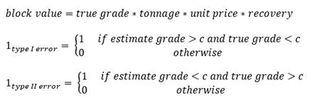
Realizations simulated with SIS showed more connectivity between high grade points than realizations simulated with SGS, as shown in Figure 2. In this case of study the difference between global interpolation errors obtained with SIS and SGS was small, as shown in Figure 3, probably due to the tight spacing of the exploration drillhole data used to generate simulations.

The estimation error increases with drillhole spacing and the average error departs from zero from 20m drillhole spacing to wider spacing (Figure 3). Interpolation errors and the economic impact of classification errors became erratic after 20 m drillhole spacing (Figures 3, 4 and 5), this could be use for exploration drillhole spacing analysis.

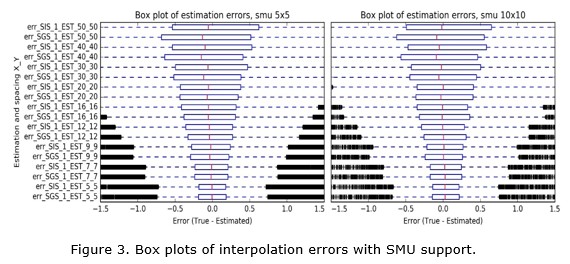
Figure 4 shows a comparison of drilling costs and misclassification costs in 5 m by 5 m by 5 m SMUs and 10 m by 10 m by 5 m SMUs. In both cases the optimum drillhole spacing would be between 5 m and 7 m.

 

 

3.2. Extra considerations

For a lower cost of drilling the optimum spacing may be too tight and operationally impossible to drill, in this case it is possible to use as reference the cost of misclassifying ore as waste and the cost of misclassifying waste as ore individually, as shown in Figure 5.

 

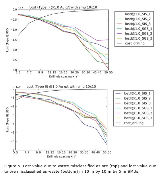
In gold deposits, where a concentration of few grams per tone represent a very high value, few SMUs may increase considerably the total lost value. One way to avoid these extreme values is by capping the lost value to a maximum, for example, Figure 6 shows the drillhole optimisation for 10 m by 10 m by 5 m SMU with capping on lost value to -10 000 USD, which is equivalent to an interpolation error of ±0,25 g/t (calculated as 10 000 USD / (10 m * 10 m * 5 m * 2,7 t/m3 *900 USD/oz * 0,0321507 oz/g) ~ 0,25 g/t ).

A more elaborated solution would be using dig lines generated with SMU’s true grades and calculating lost values only in misclassified blocks laying along dig lines contacts. An intermediate solution would be imposing diggability constraints to exclude non-minable SMUS from total lost value calculations, for example, isolated ore SMU within waste SMUs or vice versa.

4. CONCLUSIONS

Comparisons of drilling costs with misclassification costs provide an economic criterion to determine the optimum spacing between grade control drillhole drilled with reversed circulation. The method is only valid if free selection assumption is appropriated and it tends to overstate misclassification cost.

Under certain circumstances, for example, in presence of commodities with extreme value and low concentration, like gold deposits, it is important to select reasonable large SMUs and minimize the impact of extremely large errors and lost values. It is also important to consider different simulation scenarios to assess variation on results.

5. RECOMMENDATIONS

It is recommended to investigate options to impose diggability constraints on ore-waste selection to reduce the overestimation of misclassification costs, including:

· calculate lost values using only blocks misclassified along dig lines contacts.

· use connectivity parameters to exclude non-minable SMUs from total lost value calculations.

6. REFERENCES

Bertoli, O.; Paul, A.; Casley, Z. and Dunn, D. 2013: Geostatistical drillhole spacing analysis for coal resource classification in the Bowen Basin, Queensland. International Journal of Coal Geology 112: 107–113.

Boucher, A.; Dimitrakopoulos, R. and Vargas, J. A. 2005: Joint Simulations, Optimal Drillhole Spacing and the Role of the Stockpile. In: Geostatistics Banff 2004. Springer Netherlands, Dordrecht, p. 35–44. Accessed: 16 November 2016.

Chilès, J. P. and Delfiner, P. 2009: Geostatistics: Modeling Spatial Uncertainty. Wiley. Wiley Series in Probability and Statistics.

Goria, S.; Galli, A. and Armstrong, M. 2001: Quantifying the impact of additional drilling on an openpit gold project. In: 2001 annual conference of the International Association for Mathematical Geology. Cancun, Mexico.

Journel, A. G. and Kyriakidis, P. C. 2004: Evaluation of Mineral Reserves: A Simulation Approach. Oxford University Press.

Larrondo, P. 2003: Entropy of Gaussian Random Functions and Consequences in Geostatistics. Department of Civil and Environmental Engineering University of Alberta. CCG Annual Report. Available in: http://www.ccgalberta.com/ccgresources/report05/2003-129-entropy.pdf

Martínez, A. 2016: PyGSLIB. Python 2.7 package. Opengeostat Consulting. Available in: https://github.com/opengeostat/pygslib

Verly, G.; Postolski, T. and Parker, H. M. 2014: Assessing Uncertainty with Drill Hole Spacing Studies–Applications to Mineral Resources. In: Orebody Modelling and Strategic Mine Planning Symposium 2014. Australasian Institute of Mining and Metallurgy. Perth, Australia, 24-26 November.

 

 

 

Recibido: 1/12/2016
Aceptado: 6/01/2017

 

 

 

Adrian Martínez Vargas, PhD in Geological Sciences. Principal Consultant. Opengeostat Consulting, Vancouver, Canada [e-mail]

---

^[1] The notation is (dip angle --> azimuth direction).

^[2] Calculated as 10 000 USD / (10 m * 10 m * 5 m * 2,7 t/m³ *900 USD/oz * 0,0321507 oz/g) ~ 0,25 g/t.