


 Serviços customizados
 Inglês (pdf)
 Artigo em XML
 Referências do artigo
 Enviar este artigo por email
 Citado por SciELO
  Similares em
SciELO
Similares em
SciELO 
 Permalink
INTRODUCTION
The Swerling models (Swerling, 1960) were proposed as part of the broad theoretical framework dedicated to modeling the characteristics of the received radar signal and to estimate the statistical behavior of the targets radar cross section (RCS), its temporal variations as well as the detection quality. All the above elements have contributed to use these models as a typical reference to compare the performance of new detection techniques in simulations prior to any implementation. Representative examples include simulations for adaptive detection in Gaussian noise with unknown covariance matrix (Besson et al., 2015), the detection of fluctuating extended targets (Ding et al., 2017), the performance evaluation for ordered-statistic constant false alarm rate detectors (Kong et al., 2016), techniques for small and slow targets detection in marine clutter (Kemkemian et al., 2015), as well as the effectiveness evaluation of chaff recognition algorithms (Bendayan and Garcia, 2015). More recently, some generalized models have been incorporated (Meller, 2018) and even methods based directly on electromagnetic simulation of the RCS (How and Lun, 2016), however the use of these is not yet widespread.
Although several literature describes the Swerling models (Richards, 2005; Richards et al., 2010; Skolnik, 2001), most of them present the detection quality results and make little emphasis in the simulation of the radar video signal ruled by these models. Among the significant examples in this regard, we highlight the works of (Richards, 2008) and (Hughes, 2017), in addition to few functions offered by MATLAB software (MathWorks, 2017). However, the authors have not found explicit procedures and algorithms, especially useful for new researchers interested in the subject. For this reason, the two main objectives of this work are: to propose explicitly procedures that simulate the radar video signal for two types of commonly used detectors (linear and quadratic), as well as to verify that the statistical characteristics of the generated samples follows the Swerling models. In addition to the four fluctuating models, the case of non-fluctuating target is included (Marcum, 1947, 1948) because it simulation is also of interest.
The first section of this article outlines the fundamental characteristics of the Swerling models and the detectors types. Then we propose the algorithms that constitute the core of the present work and proceed to verify that the generated samples have the statistical characteristics required by the models.
MATERIALS AND METHODS
The Swerling models (Swerling, 1960, 1997) were created taking into account the common problem of detecting M received echoes. The motivation to consider this type of detection is based on the simplified model of a rotating pulse radar, in which the antenna have Ω degrees per second of angular velocity, with θ degrees of half power beamwidth through the horizontal plane and fr Hertz of pulse repetition frequency. Although a certain amount of energy is received by the antenna secondary lobes, significant echoes are received only when the target is illuminated by the main lobe, so that for each scan of 360 degrees, a packet of  pulses is received.
Each Swerling model is a combination of two probability density functions (pdf) and two decorrelation characteristics for the RCS, resulting in a total of four combinations. Swerling considered two extreme cases for decorrelation characteristics between the M pulses samples. The first case is known as scan-to-scan decorrelation or slow fluctuation, and it assumes that the M pulses amplitudes in each scan (packet) are equals, but the new M pulses amplitudes in the next scan will differ from the previous packet, so that they are independent. The second case is referred to as pulse-to-pulse decorrelation and is applicable to rapidly fluctuating targets, so that the 𝑀 pulses amplitudes within the packet are independent of each other. Before the advent of the Swerling models, the non-fluctuating target model was proposed by Marcum (Marcum, 1947, 1948), in which the pulses amplitude remains constant, so it does not vary neither between pulses nor between consecutive packets. Some authors refer to this case as Swerling 0 or Swerling 5.
The two pdf used by Swerling to describe the RCS variations are the Exponential and the 4th order Chi-square models. However, to simulate radar signals it is more useful to work directly with the echoes amplitude instead of doing so with the RCS. Since the amplitude is proportional to the square root of the RCS, it follows a Rayleigh pdf (Walck, 2007) and 4th order Chi (Walck, 2007) pdf as shown in Eq. (1) and (2) respectively (Richards et al., 2010), where the average RCS of the target is denoted as  .
.
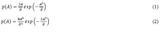
The Rayleigh model describes targets composed with several independent reflectors, none of which predominates. For its part, the Chi model describes targets with several reflectors of similar intensity and one that predominates over the others. Table 1 summarizes the characteristics of the models, denoted as Swerling 1, 2, 3 and 4.

Detectors Types
The signal received by the radar is typically a narrow band signal, modulated in amplitude, frequency and phase depending on the target characteristics. This means that the echo signal can be written as

Where At represents the envelope, f0 the carrier frequency (in most cases equal to the intermediate frequency of the receiver), the phase and n(t) is considered additive white gaussian noise (AWGN). The detector extracts the information from the received signal in order to decide if this corresponds to target or noise. In most cases, the detector is located after the intermediate frequency amplifier and its output is known as the video signal.
For the most used detection schemes, the received signal is separated in two channels as shown in Figure 1, the upper in phase channel (I) and the lower quadrature (Q) channel, here the (I/Q) detector name (Skolnik, 2001). After mixing r(t) with the local oscillator and the low pass filtering (LPF), the signals  are combined to extract the amplitude information as indicated in the figure, depending on the detector type. For the linear detector, the output is directly proportional to the envelope of the received signal, while for the quadratic detector it will be proportional to the square of the aforementioned envelope. The following section proposes the algorithms that allow us to generate the samples corresponding to the video signal for both detector types.

Algorithms to Generate the Random Samples
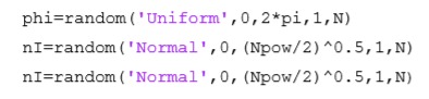
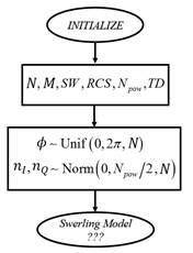
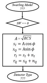
Figure 2 shows the initial procedure to establish the total number of samples to be generated N, the number of pulses received in each scan M, the Swerling model (SW), the target RCS, the total noise power (N
pow
) and the detector type (TD). From these parameters the arrays are generated, each one with N samples of the random variables corresponding to the received signal phase (with uniform distribution between 0 and 2π) and to the I and Q channels AWGN, with zero mean and variance N
pow
/2 (equal to the average noise power). Taking as representative example the use of MATLAB (MathWorks, 2017), these three arrays can be generated through the functions
are generated, each one with N samples of the random variables corresponding to the received signal phase (with uniform distribution between 0 and 2π) and to the I and Q channels AWGN, with zero mean and variance N
pow
/2 (equal to the average noise power). Taking as representative example the use of MATLAB (MathWorks, 2017), these three arrays can be generated through the functions
Afterwards, the Swerling model is verified and the algorithm goes to generate the amplitude samples with the corresponding distribution and correlation characteristics.
If it is desired to simulate a non-fluctuating target (SW = 0), the procedure shown in Figure 3 is performed. In this case, the amplitude 𝐴 of the echoes remains constant between consecutive pulses (samples) with a value equal to the square root of the RCS (Richards et al., 2010), while the phase  is the previously generated random variable. Then the noise is added to the echo components Si and Sq to create the received signal components ri and rq which will be detected by the corresponding detector in order to obtain the array with the video signal samples.
For the slow fluctuation models of Swerling 1 and 3, the generated samples follow the procedure of Figure 4. Depending on the model, the amplitude of the echo will be ruled by the Rayleigh pdf for Swerling 1, or by the 4th order Chi pdf for Swerling 3.
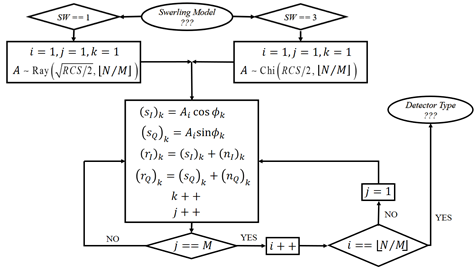
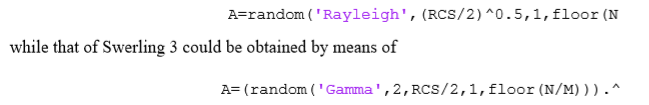
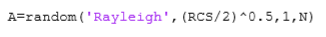
Taking MATLAB as example again, the amplitude samples that follow the Swerling 1 model could be generated by the function
In each case the number of samples is the smallest and closest integer to N/M, with the aim of simulating the packet of equal amplitude for each scan, which constitutes the scan-to-scan decorrelation model or slow fluctuation (Richards, 2008; Richards et al., 2010). For the proposed procedure, the counter 𝑖 represents the packet index, j indicates if the M pulses of equal amplitude within the packet were generated, while k is used as counter for the samples total.
Similarly, the samples for Swerling 2 and 4 models are generated following the procedure of Figure 5. The difference with respect to the previous case is that a different sample is generated for each pulse, which constitutes the pulse-to-pulse decorrelation or fast fluctuation model (Richards, 2008; Richards et al., 2010).
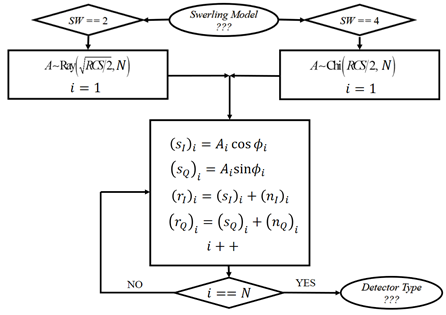
From the figure, the meaning of i is clear as index for the individual samples. With MATLAB, the functions that could be used to generate the array of N elements for Swerling 2 could be
Where as in the case of Swerling 4 it could be

As before, once generated the samples the detector type is determined. Depending on the selected detector type (TD = 0 for linear and TD = 1 for quadratic) and taking into account the diagram of Figure 1, the received signal components are combined as indicated in Figure 6 to obtain the video signal vs. The vn array contains only noise samples that could be used with other purposes in simulations. An example of the latter would be the DRACEC method (Chávez and Guillén, 2018), where separate noise samples are required to simulate the background and anomaly classes.

Verification of the Samples Statistical Characteristics
Figure 7 and Figure 8 show the estimated pdfs of the pulse amplitude generated with the above mentioned functions through MATLAB (MathWorks, 2017). It is shown in blue the pdfs estimate by histograms, while in red its fit to Eq. (1) and Eq. (2). Besides Table 2 shows the fit quality of all the generated random variables taking into account several numeric indicators described below.

Fig. 7 Pulse amplitude pdf estimated by histograms (blue) and its fit (red) to the Rayleigh pdf of Eq. (1) (Swerling 1 and 2).
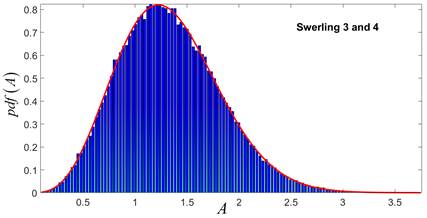
Fig. 8 Pulse amplitude pdf estimated by histograms (blue) and its fit (red) to 4th order Chi pdf of Eq. (2) (Swerling 3 and 4).
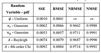
The coefficient SSE is the sum of squared errors of the fit and is defined by Eq. (4) (MathWorks, 2017), so a value close to zero indicates that the estimated pdf is well fitted (see Table 2). Henceforward 𝑦i represents the estimated pdf values while  denotes the fit values.

The RMSE is the root mean square error of the fit and is determined by Eq. 5 (MathWorks, 2017). A value close to zero indicates a good fit quality (see Table 2).

Finally, the NRMSE and NMSE indicators are calculated using Eq. (6) and Eq. (7) (MathWorks, 2017), which take values between -∞ (bad fit) and unity (perfect fit). The value of these coefficients is not useful to analyze the fit quality of  to the uniform pdf, because when the fit is a constant, it coincides with its average value
  , causing the denominator of both equations going to zero and therefore both indicators tend to -∞ (see Table 2).

CONCLUSIONS
Through the proposed algorithms it is possible to generate samples of the video signal following the four Swerling models in addition to the non-fluctuating target case. Although the functions to generate the random samples were exemplified using MATLAB, the algorithms implementation is not limited to this tool, since its general nature makes it possible to develop them in any software platform.
On the other hand, the probability densities of the amplitude and phase of the simulated echoes, as well as the AWGN noise taken as interference, were fitted with a high quality to the assumed models. In addition, the provided procedures are easily reproducible, which decreases the development time of the simulations prior to any real implementation, especially for new researchers interested in generating samples of the video signal for the linear and quadratic detectors.

